
Mississippi State University Mississippi State University
Scholars Junction Scholars Junction
Theses and Dissertations Theses and Dissertations
8-6-2011
An open virtual testbed for industrial control system security An open virtual testbed for industrial control system security
research research
Bradley Galloway Reaves
Follow this and additional works at: https://scholarsjunction.msstate.edu/td
Recommended Citation Recommended Citation
Reaves, Bradley Galloway, "An open virtual testbed for industrial control system security research" (2011).
Theses and Dissertations
. 613.
https://scholarsjunction.msstate.edu/td/613
This Graduate Thesis - Open Access is brought to you for free and open access by the Theses and Dissertations at
Scholars Junction. It has been accepted for inclusion in Theses and Dissertations by an authorized administrator of
Scholars Junction. For more information, please contact [email protected].
AN OPEN VIRTUAL TESTBED FOR INDUSTRIAL CONTROL SYSTEM
SECURITY RESEARCH
By
Bradley Galloway Reaves
A Thesis
Submitted to the Faculty of
Mississippi State University
in Partial Fulfillment of the Requirements
for the Degree of Master of Science
in Computer Engineering
in the Department of Electrical and Computer Engineering
Mississippi State, Mississippi
August 2011
Copyright by
Bradley Galloway Reaves
2011

AN OPEN VIRTUAL TESTBED FOR INDUSTRIAL CONTROL SYSTEM
SECURITY RESEARCH
By
Bradley Galloway Reaves
Approved:
Thomas Morris
Assistant Professor of Electrical and
Computer Engineering
(Major Professor)
Yoginder Dandass
Associate Professor of Computer
Science and Engineering
(Committee Member)
Rayford B. Vaughn
Associate Vice President for Research,
Professor of Computer Science and Engi-
neering
(Committee Member)
James Fowler
Professor of Electrical and
Computer Engineering,
Graduate Coordinator
Sarah A. Rajala
Dean of the James Worth Bagley College
of Engineering
Name: Bradley Galloway Reaves
Date of Degree: August 6, 2011
Institution: Mississippi State University
Major Field: Computer Engineering
Major Professor: Dr. Thomas Morris
Title of Study: AN OPEN VIRTUAL TESTBED FOR INDUSTRIAL CONTROL
SYSTEM SECURITY RESEARCH
Pages in Study: 144
Candidate for Degree of Master of Science
ICS security has been a topic of scrutiny and research for several years, and many
security issues are well known. However, research efforts are impeded by a lack of an
open virtual industrial control system testbed for security research. This thesis describes a
virtual testbed framework using Python to create discrete testbed components (including
virtual devices and process simulators). This testbed is designed such that the testbeds are
interoperable with real ICS devices and that the virtual testbeds can provide comparable
ICS network behavior to a laboratory testbed. Two testbeds based on laboratory testbeds
have been developed and have been shown to be interoperable with real industrial control
system equipment and vulnerable to attacks in the same manner as a real system. Addition-
ally, these testbeds have been quantitatively shown to produce traffic close to laboratory
systems (within 90% similarity on most metrics).
DEDICATION
To Sarah.
ii
ACKNOWLEDGMENTS
This thesis would not be possible without the support of a number of people. I would
first like to thank my advisor, Dr. Thomas Morris, for his help and guidance over the
years. I would also like to thank Dr. Dandass and Dr. Vaughn for their encouragement and
helpful advice.
Discussions with Jacob Brodsky about wireless insecurity and ICS security in gen-
eral were enlightening. Terry Brugger provided source code which inspired my imple-
mentation of similarity metrics. Wei Gao’s help with maintaining the MSU ICS security
laboratory and attack code is greatly appreciated.
This material is based upon work supported by the National Science Foundation Grad-
uate Research Fellowship under Grant No. DEG-1125191.
iii
TABLE OF CONTENTS
DEDICATION . . . . . . . . . . . . . . . . . . . . . . . . . . . . . . . . . . . . ii
ACKNOWLEDGMENTS . . . . . . . . . . . . . . . . . . . . . . . . . . . . . . . iii
LIST OF TABLES . . . . . . . . . . . . . . . . . . . . . . . . . . . . . . . . . . vii
LIST OF FIGURES . . . . . . . . . . . . . . . . . . . . . . . . . . . . . . . . . . viii
LIST OF APPREVIATIONS . . . . . . . . . . . . . . . . . . . . . . . . . . . . . x
CHAPTER
1. INTRODUCTION . . . . . . . . . . . . . . . . . . . . . . . . . . . . . . 1
1.1 Motivation . . . . . . . . . . . . . . . . . . . . . . . . . . . . . . . 1
1.1.1 Problems in ICS Security . . . . . . . . . . . . . . . . . . . . 1
1.1.2 Problems Faced by ICS Security Research . . . . . . . . . . 3
1.1.3 Need for an open testbed for ICS security development . . . . 5
1.2 Contribution . . . . . . . . . . . . . . . . . . . . . . . . . . . . . . 8
2. RELATED WORK . . . . . . . . . . . . . . . . . . . . . . . . . . . . . . 11
2.1 Industrial Control Systems . . . . . . . . . . . . . . . . . . . . . . . 11
2.1.1 Programmable Logic Controllers . . . . . . . . . . . . . . . 12
2.1.2 ICS Protocols . . . . . . . . . . . . . . . . . . . . . . . . . . 13
2.1.2.1 Modbus . . . . . . . . . . . . . . . . . . . . . . . . 14
2.1.2.2 HART . . . . . . . . . . . . . . . . . . . . . . . . . 16
2.2 Related Testbeds . . . . . . . . . . . . . . . . . . . . . . . . . . . . 16
2.2.1 MSU Lab . . . . . . . . . . . . . . . . . . . . . . . . . . . . 18
2.3 Intrusion Detection Systems . . . . . . . . . . . . . . . . . . . . . . 20
2.3.1 IDS Testing . . . . . . . . . . . . . . . . . . . . . . . . . . . 22
2.4 PCS IDS . . . . . . . . . . . . . . . . . . . . . . . . . . . . . . . . 23
3. SURVEY OF ICS WIRELESS ATTACK LITERATURE . . . . . . . . . . 25
iv
3.1 IEEE 802.11 . . . . . . . . . . . . . . . . . . . . . . . . . . . . . . 26
3.2 IEEE 802.15.4 PHY and MAC Layer . . . . . . . . . . . . . . . . . 33
3.3 WirelessHART . . . . . . . . . . . . . . . . . . . . . . . . . . . . . 36
3.4 ZigBee . . . . . . . . . . . . . . . . . . . . . . . . . . . . . . . . . 40
3.5 Proprietary Wireless . . . . . . . . . . . . . . . . . . . . . . . . . . 43
3.6 Bluetooth . . . . . . . . . . . . . . . . . . . . . . . . . . . . . . . . 46
4. OVERVIEW OF VIRTUAL TESTBED . . . . . . . . . . . . . . . . . . . 51
4.1 Design Goals of Virtual Testbed . . . . . . . . . . . . . . . . . . . . 52
4.2 Components . . . . . . . . . . . . . . . . . . . . . . . . . . . . . . 54
4.2.1 Process Simulator . . . . . . . . . . . . . . . . . . . . . . . 57
4.2.2 Virtual Devices . . . . . . . . . . . . . . . . . . . . . . . . . 57
4.2.3 Configuration Files . . . . . . . . . . . . . . . . . . . . . . . 58
4.3 Use Cases . . . . . . . . . . . . . . . . . . . . . . . . . . . . . . . . 59
4.4 Logging . . . . . . . . . . . . . . . . . . . . . . . . . . . . . . . . . 61
4.4.1 TCP/IP Logging . . . . . . . . . . . . . . . . . . . . . . . . 61
4.4.2 Serial System Logging . . . . . . . . . . . . . . . . . . . . . 62
4.5 Testbed Systems . . . . . . . . . . . . . . . . . . . . . . . . . . . . 64
4.5.1 Pipeline . . . . . . . . . . . . . . . . . . . . . . . . . . . . 64
4.5.2 Ground Tank . . . . . . . . . . . . . . . . . . . . . . . . . . 65
5. PROCESS SIMULATORS . . . . . . . . . . . . . . . . . . . . . . . . . . 66
5.1 Design . . . . . . . . . . . . . . . . . . . . . . . . . . . . . . . . . 67
5.2 Simulated Systems . . . . . . . . . . . . . . . . . . . . . . . . . . . 71
5.3 How to create a new simulation . . . . . . . . . . . . . . . . . . . . 72
6. VIRTUAL ICS DEVICES . . . . . . . . . . . . . . . . . . . . . . . . . . 78
6.1 Design . . . . . . . . . . . . . . . . . . . . . . . . . . . . . . . . . 79
6.1.1 Points . . . . . . . . . . . . . . . . . . . . . . . . . . . . . . 80
6.1.2 Control Logic . . . . . . . . . . . . . . . . . . . . . . . . . . 83
6.1.3 Simulator interface . . . . . . . . . . . . . . . . . . . . . . . 84
6.1.4 ICS protocol interfaces . . . . . . . . . . . . . . . . . . . . . 86
6.1.4.1 Modbus Implementation . . . . . . . . . . . . . . . 88
6.2 Implementing a vdev . . . . . . . . . . . . . . . . . . . . . . . . . . 91
7. EVALUATION . . . . . . . . . . . . . . . . . . . . . . . . . . . . . . . . 93
7.1 Virtual Testbed Integration with Actual ICS Devices . . . . . . . . . 94
7.1.1 Integration with ICS Radio . . . . . . . . . . . . . . . . . . . 94
7.1.2 Integrating a Virtual Devices with Actual Devices . . . . . . . 98
v
7.2 Virtual Testbed under Attack . . . . . . . . . . . . . . . . . . . . . . 99
7.3 Traffic Fidelity Analysis . . . . . . . . . . . . . . . . . . . . . . . . 108
7.3.1 Methodology . . . . . . . . . . . . . . . . . . . . . . . . . . 108
7.3.1.1 Mathematics . . . . . . . . . . . . . . . . . . . . . 109
7.3.1.2 ModbusRTU Metrics . . . . . . . . . . . . . . . . . 111
7.3.2 Results . . . . . . . . . . . . . . . . . . . . . . . . . . . . . 113
7.3.2.1 Ground Tank System . . . . . . . . . . . . . . . . . 114
7.3.2.2 Pipeline System . . . . . . . . . . . . . . . . . . . . 116
8. CONCLUSIONS . . . . . . . . . . . . . . . . . . . . . . . . . . . . . . . 120
8.1 Contributions . . . . . . . . . . . . . . . . . . . . . . . . . . . . . . 120
8.2 Future work . . . . . . . . . . . . . . . . . . . . . . . . . . . . . . . 122
REFERENCES . . . . . . . . . . . . . . . . . . . . . . . . . . . . . . . . . . . . 124
APPENDIX
A. TIMING CALIBRATION . . . . . . . . . . . . . . . . . . . . . . . . . . 130
A.1 Timing calibration method for ModbusRTU systems . . . . . . . . . 131
A.2 Calibration Example: Ground Tank System . . . . . . . . . . . . . . 134
A.2.1 Initial Similarity Scores . . . . . . . . . . . . . . . . . . . . 134
A.2.2 Communications delay . . . . . . . . . . . . . . . . . . . . . 135
A.2.3 Message Processing Delay . . . . . . . . . . . . . . . . . . . 136
A.2.4 Master Program Scan Time . . . . . . . . . . . . . . . . . . 137
vi
LIST OF TABLES
2.1 Sample Modbus Function Codes . . . . . . . . . . . . . . . . . . . . . . . . 15
2.2 IDS performance metrics . . . . . . . . . . . . . . . . . . . . . . . . . . . . 21
3.1 IEEE 802.11 Vulnerabilities . . . . . . . . . . . . . . . . . . . . . . . . . . 27
3.2 IEEE 802.15.4 Vulnerabilities . . . . . . . . . . . . . . . . . . . . . . . . . 33
3.3 WirelessHART Vulnerabilities . . . . . . . . . . . . . . . . . . . . . . . . . 37
3.4 ZigBee Vulnerabilities . . . . . . . . . . . . . . . . . . . . . . . . . . . . . 40
3.5 Example Proprietary Wireless Systems . . . . . . . . . . . . . . . . . . . . . 44
3.6 Proprietary Wireless System Vulnerabilities . . . . . . . . . . . . . . . . . . 45
7.1 Similarity Metrics for Ground Tank (Off) Connected with Radios . . . . . . . 96
7.2 Similarity Metrics for Ground Tank (Auto) Connected with Radios . . . . . . 97
7.3 Similarity Metrics For the Ground Tank System(Off Mode) . . . . . . . . . . 115
7.4 Similarity Metrics For the Ground Tank System(Auto Mode) . . . . . . . . . 116
7.5 Similarity Metrics For the Pipeline System (Auto Mode) . . . . . . . . . . . 117
7.6 Similarity Metrics For the Pipeline System (Off Mode) . . . . . . . . . . . . 118
A.1 Ground Tank Initial Similarity Scores . . . . . . . . . . . . . . . . . . . . . 135
A.2 Ground Tank Similarity Scores After Adding Baud Rate Delay . . . . . . . . 136
A.3 Ground Tank Similarity Scores After Message Processing Delay . . . . . . . 141
A.4 Ground Tank Similarity Scores After Adjusting Master Scan Time . . . . . . 144
vii
LIST OF FIGURES
2.1 Diagram of an ICS System . . . . . . . . . . . . . . . . . . . . . . . . . . . 12
4.1 Testbed Architecture . . . . . . . . . . . . . . . . . . . . . . . . . . . . . . 55
5.1 Simulator Architecture . . . . . . . . . . . . . . . . . . . . . . . . . . . . . 68
5.2 Ground Tank Empty to Full . . . . . . . . . . . . . . . . . . . . . . . . . . . 73
5.3 Ground Tank Full to Empty . . . . . . . . . . . . . . . . . . . . . . . . . . . 74
5.4 Ground Tank Simulation Comparisons: Ground Tank Auto Mode . . . . . . . 75
5.5 Pressures of Pipeline Systems in Auto Mode . . . . . . . . . . . . . . . . . . 76
6.1 Virtual Device Architecture . . . . . . . . . . . . . . . . . . . . . . . . . . . 80
6.2 Sample Process Control Logic . . . . . . . . . . . . . . . . . . . . . . . . . 84
7.1 Virtual Device Radio Integration Testing . . . . . . . . . . . . . . . . . . . . 95
7.2 Real Device Interoperability Test Setups . . . . . . . . . . . . . . . . . . . . 98
7.3 One Hertz Injection Attack Setup . . . . . . . . . . . . . . . . . . . . . . . . 100
7.4 Virtual System Tank Levels During Injection Attack . . . . . . . . . . . . . . 102
7.5 Laboratory System Tank Levels During Injection Attack . . . . . . . . . . . 103
7.6 Virtual Pipeline Pressures During Radio DoS Attack . . . . . . . . . . . . . . 104
7.7 Laboratory Pipeline Pressures During Radio DoS Attack . . . . . . . . . . . 105
7.8 Virtual Pipeline Pressures Received During Radio DoS/Injection Attack . . . 106
7.9 Laboratory Pipeline Pressures Received During Radio DoS/Injection Attack . 107
viii
A.1 Master-Slave Interarrival Distribution (Write Command) . . . . . . . . . . . 138
A.2 Master-Slave Interarrival Distribution (Read Command) . . . . . . . . . . . . 139
A.3 Master-Slave Interarrival Distribution (Read) After Processing Delay . . . . . 140
A.4 Ground Tank Master-Master Interarrival Time Before Adding Delay . . . . . 142
A.5 Plot of Interarrival Distribution After Calibration . . . . . . . . . . . . . . . 143
ix
LIST OF APPREVIATIONS
AES — Advanced Encryption Standard
ARP — Address Resolution Protocol
CAC — Bluetooth Channel Access Code
AES-CBC — AES Cipherblock Chaining Mode
CCA — Clear Channel Assessment
MS-CHAP — Microsoft Challenge Handshake Authentication Protocol
CRC — Cyclic Redundancy Check
CSV — Comma Separated Value file
AES-CTR — AES Counter Mode
DCS — Distributed Control System
DMZ — DeMilitarized Zone
DNP3 — Distributed Network Protocol 3
DNS — Domain Name System
EAP — Extensible Authentication Protocol
x
EAP-TTLS — Extensible Authentication Protocol Tunneled Transport Layer Security
ECDH — Elliptic Curve Diffie-Hellman
FHSS — Frequency Hopping Spread-Spectrum
FTP — File Transfer Protocol
GTK — Group Temporal Key
GUI — Graphical User Interface
HART — Highway Addressible Remote Transducer protocol
HMI — Human Machine Interface
HTTP — HyperText Transfer Protocol
ICS — Industrial Control System
IDS — Intrusion Detection System
IP — Internet Protocol
ISM — Industrial, Scientific, Medical RF Frequency Band
JSON — JavaScript Object Notation
LAN — Local Area Network
LAND — Local Area Network Denial attack
LEAP — Lightweight Extensible Authentication Protocol
xi
MAC — Medium Access Control (network layer) or Message Authentication Code
MD5 — Message Digest 5 Hash Algorithm
MIC — Message Integrity Code
MITM — Man-in-the-Middle attack
MTU — Master Terminal Unit
NERC — North American Electric Reliability Corporation
PAC — Programmable Automation Controller
PAN — Personal Area Networks
PCAP — Packet Capture (file format)
PCS — Process Control System
PDC — Phasor Data Concentrator
PEAP — Protected Extensible Authentication Protocol
PID — Proportional-Integral-Derivative control scheme
PLC — Programmable Logic Controller
PMU — Phasor Measurement Unit
PSK — Pre-Shared Key (IEEE 802.11)
PTK — Pairwise Transient Key
xii
RADIUS — Remote Authentication Dial-In User Service
RC4 — Rivest Cipher 4 stream cipher
RTDS — Real Time Digital Simulator
RTU — Remote Terminal Unit
SCADA — Supervisory Control And Data Acquisition
SIFS — Short Interframe Space (IEEE 802.11)
SKKE — Symmetric-Key Key Exchange
SPAN — Switched Port Analyzer
SSID — Service Set Identifier
SSP — Secure Simple Pairing
TCP — Transmission Control Protocol
TDMA — Time Domain Multiple Access
TKIP — Temporal Key Integrity Protocol
TTL — Time-to-Live (counter in IP headers)
UDP — User Datagram Protocol
USRP — Universal Software Radio Peripheral
VLAN — Virtual LAN
xiii
VPN — Virtual Private Network
WEP — Wired-Equivalent Privacy
WPA — WiFi Protected Access
WPA2 — WiFi Protected Access 2
xiv
CHAPTER 1
INTRODUCTION
1.1 Motivation
1.1.1 Problems in ICS Security
Industrial Control Systems (ICS), also known as Distributed Control Systems (DCS),
Process Control Systems (PCS), and Supervisory Control and Data Acquisition (SCADA)
systems are computer systems used to monitor control physical processes in manufac-
turing, chemical processing, electric generation, electric transmission and distribution,
water/wastewater systems, and other industries. PCS collect data from remote facilities
about the state of the physical process and send commands to control the physical process.
Process control system communications are characterized by mainly machine-to-machine
communications in point-to-point links and networks consisting of mainly computation-
ally limited devices.
ICS security has been a topic of scrutiny and research for several years, and many secu-
rity issues are well known[21, 22]. First, ICS often have poor security policies, including
not enforcing strong, secret passwords for individual users. Second, human-machine in-
terface software has been shown to have major flaws in user authentication [48]. Third,
ICS communication protocols provide no mechanisms to guarantee integrity, authenticity,
1
or confidentiality of data, making injection or tampering of ICS communications possi-
ble (and in some cases, trivial). This is made worse by the fact that while historically
ICS were directly connected using serial and fieldbus protocols, new advances in Ether-
net and TCP/IP networking used in enterprise networks have become integrated into ICS
networks. These advances allow previously separate ICS and enterprise networks to be
bridged, allowing attackers of the enterprise network potential access to the ICS network
as well.
Moreover, operators are reticent to patch ICS devices as patching requires downtime,
and patches may break currently working systems; ICS, despite the reliability of the in-
dustrial hardware, are quite difficult to operate and maintain. As such, ICS operators are
reticent to change anything in a working system. Some ICS devices use commercial off-
the-shelf operating systems, including Microsoft Windows. These devices are vulnerable
to attacks against these operating systems in the same way as PCs. Other systems use cus-
tom embedded or real-time operating systems; these proprietary systems are less tested for
vulnerabilities by product developers, security researchers, and hackers, and may harbor
many common programming and design errors like buffer overflows. For example, labo-
ratory testing of ICS equipment has shown some devices to be vulnerable to common TCP
SYN flood and LAND attacks; these vulnerabilities are no longer present in commodity
operating system network stacks.
Much of the current research focuses on TCP/IP-based networks, and as such there
is an emphasis on securing so-called “routable” protocols and ignoring “non-routable”
protocols. Non-routable protocols are believed to be secure against any attacker without
2
physical access. The NERC Critical Infrastructure Protection [8] requirements show this
philosophy in action. While it is, in fact, impractical to attack non-routable systems that
use, for example, RS-232 connections without physical access, industrial wireless sys-
tem use is becoming more and more prevalent in both routable and non-routable systems.
These wireless systems introduce a number of vulnerabilities that can be exploited by
attackers.
Additionally, these wireless systems sometimes make non-routable systems routable,
and in all cases there is a greater risk of attack as attackers no longer need physical access
to the systems to attack them because they can be attacked beyond logical boundaries
(connection points). As an example of this, attackers may jam, eavesdrop, or inject packets
between two wireless radios that are within a security perimeter, even in a secure building.
This greatly complicates the concept of security perimeter, and even more challenges the
assumption that non-routable systems are not in need of additional security practices. This
is discussed further in Chapter 3.
1.1.2 Problems Faced by ICS Security Research
As discussed in the previous section, the development of security practices and tech-
niques in the realm of process control systems has lagged the development seen in tra-
ditional information technology. However, researchers and industry practitioners have
taken notice of the issue and are developing best practices, secure protocols[46, 32], and
intrusion detection systems to meet the security needs of industrial control systems. Re-
searchers have explored a number of different approaches to performing intrusion detec-
3
tion in process control systems, including signature-based, anomaly-based, model-based,
state-based, and hybrid techniques. These will be discussed in further detail in the related
work. However, research efforts are hampered by a number of issues.
First, industrial control systems are quite diverse in network size and topology, the
number of standard communication protocols, communications media, as well as types of
process to be controlled. Presently, researchers are only able to test their work in their own
laboratory testbeds, which are necessarily limited in size and scope and not able to exhibit
the diversity seen in real-world applications.
A second issue to ICS research follows from the first: it is difficult for researchers
to develop generic solutions that can be used in many different process control systems
because of their limited test systems. The solutions designed often only work given certain
assumptions about the ICS system configuration, and reported results can only be provided
in terms of the single system it was tested in.
Third, many of these testbeds are actually simulations developed in common network
simulation toolkits like OmNet++ or NS2. These are purely simulated systems, and no
work has been done to measure the similarity of the results of this traffic compared to actual
ICS. Research results from these testbeds are dependent on fundamental assumptionsmade
by the testbed designers, which may or may not hold true in practice. This limits the types
of possible research approaches and the trustworthiness of the results.
The fourth issue is a grave problem for the scientific process: in some cases, solu-
tions developed in one testbed are not easily distributed and tested in a different testbed
for comparison. This means that, at present, it is difficult to quantitatively compare differ-
4
ent approaches directly to determine which approaches are more promising and effective.
Currently, there is no “standard” test scenario for ICS security solutions.
1.1.3 Need for an open testbed for ICS security development
There are two approaches to creating a testbed: laboratory-scale ICS with real equip-
ment and virtual testbeds. Some researchers use small, laboratory-scale processes con-
trolled by ICS consisting of a few devices. Other researchers use virtual testbeds; these
consist of simulated ICS devices, and may include a simulated process as well.
Laboratory scale systems have a number of advantages compared to virtual systems.
First, the data will reflect realistic measurement variations that would be present in an ac-
tual process control system. Second, the communication patterns and latencies will be en-
tirely accurate and not vulnerable to inaccuracies in simulated variables like OS scheduling
load. Third, PCS devices are individually vulnerable to many attacks that may not affect all
systems. These vulnerabilities may not be present in the specification of the system that the
virtual testbed was designed to emulate; examples include protocol implementation bugs
that cause the device to be vulnerable to Teardrop attacks, LAND attacks, web application
attacks, or buffer overflows. Other security issues like poorly protected or hard-coded de-
fault passwords to devices will also not be present. With laboratory scale process control
systems, captures of these attacks can be provided in addition to protocol-based attacks
and normal background traffic.
In spite of their benefits, laboratory scale systems have a number of disadvantages.
First, laboratory-scale systems are expensive to develop and can be difficult to maintain.
5
In particular, ICS software can be brittle and not user-friendly, and laboratory scale pro-
cesses require maintenance to stay operational. Second, adding or changing features in
a laboratory-scale system can be difficult. Third, the size of laboratory-scale systems is
limited by the required space and funds, so by necessity the systems will be smaller and
less featured than a real ICS.
Virtual systems, on the other hand, can be simpler to develop and have practically no
maintenance costs. Doubling the size of a virtual system requires only development time,
not a large purchase order. Furthermore, virtual system configurations can be backed up
and recalled instantly, so changing or adding features to a virtual testbed after does not
permanently alter the system. However, making changes or adding features to a virtual
system is arguably easier than in a laboratory system. While the captures taken from ei-
ther a laboratory or a virtual ICS may be distributed, a major advantage of a virtual system
is that a virtual system can be distributed widely to many researchers. For example, re-
searchers may use a virtual testbed provided by another group to place intrusion prevention
systems in the testbed to test effectiveness; such distribution is impossible with laboratory
testbeds. Being able to distribute the virtual testbed also means that any researcher can
recreate traffic captures if necessary; such capture regeneration may be necessary if bi-
ases or problems are found with previously released datasets. This openness can help the
testbed and datasets avoid obsolescence. Virtual testbeds are also more convenient to use
than laboratory testbeds for developing and debugging ICS security projects because they
are portable and require little set up for an experiment. While virtual testbeds provide a
number of benefits, there are some disadvantages to their use. Certain attacks, especially
6
attacks that rely on device implementation errors, may not work against virtual testbeds.
Also, virtual systems may not perfectly exhibit the same behavior as a real ICS system.
In spite of the advantages of a laboratory testbed, a virtual testbed that is open and
freely available will solve the four problems described in the last section.
First, an open testbed will reduce duplication of effort as research groups do not have to
all create their own testbeds; rather, if the open testbed does not fit a group’s needs it may
be improved in less time than creation of a new testbed. This results in a higher quality
testbed for all researchers with less effort. Additionally, other researchers may contribute
virtualized versions of their laboratory testbeds for all to use. By enabling the creation of
more diverse testbeds, the first two problems of the previous section can be solved.
Second, an open testbed provides a common ground for research; even if researchers
wish to use their existing testbeds, they can also test and distribute projects in the open
testbed. The benefit of this is that research groups can share code, and published results
can be duplicated and compared. This solves the fourth issue discussed in the previous
section.
Third, this testbed may be used to generate captures of normal system network traffic
and captures of attack or anomalous traffic for IDS researchers. These captures may be
distributed with or independently of the testbed itself. This is a benefit to IDS researchers
who prefer to work with captures instead of live testbeds. If the system is open, distributed
captures may be recreated to correct for unexpected biases. This reduces the possibility of
capture obsolescence.
7
Fourth, an open testbed opens the ICS security research area to more groups. Presently,
ICS research requires substantial investment. With an open testbed, researchers can ex-
plore the area without having to purchase large laboratory setups. Additionally, amateur
researchers and students can use the testbed without having to have the backing of a large
organization.
Finally, while this thesis will later describe verification of the virtual testbed, an open
testbed can be audited and verified by anyone. Because problems may be identified easier
(according to the adage “Many eyes make bugs shallow”), and corrected by any inclined
researcher, the third issue of the previous section is solved.
While the testbed can be used to address prior problems, additional features can extend
its usefulness. First, interoperability of the virtual system with actual ICS equipment will
allow for hybrid testbeds and extend the usefulness of the virtual testbed. Second, design-
ing the testbed such that important characteristics like ICS protocols or communications
interfaces can be changed will greatly enhance the ease of use of the system, especially
compared with laboratory systems. Third, designing the testbed such that components can
be replaced or extended easily will encourage use, reuse, and contribution to the testbed.
1.2 Contribution
In response to this problems discussed previously, this thesis forms the following hy-
pothesis:
It possible to:
1. Create a virtual testbed frameworkusing Python to create discrete testbed
components
8
2. that is designed such that the testbeds are interoperable with real ICS
devices and
3. that virtual testbeds can provide comparable (within 90% similarity) ICS
network behavior to a laboratory testbed.
The first clause of the hypothesis indicates that instead of a single, monolithic testbed,
a framework will be created to allow for the construction of many independent testbeds;
this framework will consist of discrete, replaceable components. From the second clause,
the created testbeds will be interoperable with real ICS devices; this extends the usefulness
of the virtual testbed, but also serves as a guarantee of realism — a virtual testbed that is
not similar to a real ICS will not be interoperable. The third clause indicates that the
virtual testbed behavior (especially with respect to network traffic) will be very similar to
laboratory testbeds; this is defined in greater detail in Chapter 7.
This thesis describes the development and evaluation of an open virtual testbed frame-
work to test this hypothesis. The design of the virtual testbed framework is broken up
into discrete components. The main components are the process simulator and the virtual
device; other components include a module for analyzing packet captures and a module
for logging and creating virtual serial ports. Two simulated systems have been created for
the testbed, and both have been designed to match existing laboratory testbeds in the MSU
laboratory (Described in Subsection 2.2.1). These are the laboratory-scale pipeline and
ground tank.
The following chapters detail the contribution of this thesis. Chapter 2 provides a
summary of related work, including more information about ICS, IDS, and related testbed
projects. Chapter 3 provides a survey of known attacks against common ICS wireless
9
systems to show how ICS wireless systems can be used to violate security assumptions
in ICS; this motivates the need for further security research in ICS, particularly in IDS.
Chapter 4 provides an overview of the virtual testbed design goals, components, use cases,
and the two implemented systems. Chapter 5 discusses process simulation, while Chapter
6 describes the design of virtual ICS devices for the testbed. Chapter 7 discusses the
verification methodology, and verification results, and use of the testbed. Finally, Chapter
8 provides conclusions and future work.
10
CHAPTER 2
RELATED WORK
2.1 Industrial Control Systems
Industrial Control Systems (ICS), also known as Distributed Control Systems (DCS),
Process Control Systems (PCS), and Supervisory Control and Data Acquisition (SCADA)
systems are computer systems used to monitor control physical processes in manufac-
turing, chemical processing, electric generation, electric transmission and distribution,
water/wastewater systems, and other industries. ICS interconnect and monitor physical
processes. An example ICS system is shown in 2.1.
ICS collect data from remote facilities about the state of the physical process and send
commands to control the physical process creating a feedback control loop. At the center
of Figure 2.1 is the Master ICS computer, termed the Master Terminal Unit (MTU). The
MTU may be a personal computer or a programmable logic controller (PLC). The MTU
interfaces with Human Machine Interface (HMI) software, and may also connect to a
historian server (not shown) or the company’s corporate network to allow engineers and
managers access to information about ongoing processes. The master unit is connected
to Remote Terminal Units (RTU), which may be termed “slaves” in some systems and
protocols. RTU may be smart instruments themselves or computers or PLCs that interface
with instruments, sensors, and actuators. Legacy ICS are connected over RS-232, RS-485,
11

Figure 2.1
Diagram of an ICS System
and other directly connected physical media. Modern ICS can incorporate those media
with Ethernet, Internet Protocol (IP), TCP, and/or UDP, and may be directly connected
to the Internet, or connected to corporate intranets which may have connections to the
Internet. In addition to the wired media of RS-232, RS-485, CANBUS, and Ethernet,
ICS systems make use of a plethora of standards-based and proprietary short-range and
long-range wireless protocols.
2.1.1 Programmable Logic Controllers
PLCs are digital computer systems that are designed to run industrial control systems.
They feature robust, rugged physical designs to withstand rough industrial environments,
and typically run embedded system or custom operating systems.Their primary purpose
12
is to send analog and digital control signals to physical equipment, The values of these
control signals will be based on the PLC programming and analog and digital inputs.PLCs
are primarily programmed using a graphical programming language known as “ladder
logic,” which emulates the original control system paradigm of using physical relays to
automate processes. However, they may also be programmed in a high-level programming
language, such as C. Once programmed, PLC programming rarely changes. PLCs run a
processing loop that consists of reading inputs, running ladder logic, and updating outputs
appropriately.A single run of this loop is known as a “scan,” and the time from the start of
one loop run to the next is known as the “scan time”
2.1.2 ICS Protocols
This section details two commonly used standards-based application protocols in ICS
systems: Modbus and HART. These protocols are used to communicate between RTU’s,
MTU’s, HMI software, and other ICS devices. Many ICS application communication
protocols, including the ones listed here, lack authentication features to prove the origin or
freshness of network traffic. This lack of authentication capability leads to the potential for
external network penetrators or disgruntled insiders to inject false data and false command
packets into a SCADA system either through direct creation of such packets or replay
attacks. These attacks may take place in either a wired or wireless context.
13
2.1.2.1 Modbus
Modbus[54] is a common protocol used in industrial control systems and SCADA sys-
tems. Modbus uses a master-slave paradigm for communications. Within Modbus, there
is no authentication of masters or slaves. Modbus may be carried over serial connections
(RS-232 or RS-485) or may be carried over TCP/IP, which is known as Modbus/TCP[55].
The Modbus data model considers data elements as being stored in four tables, each
consisting of: discrete inputs (1-bit) , coils (1-bit outputs), input registers (16-bit), and
holding registers (16-bit). Discrete inputs and input registers are read-only, and the data
comes from the device’s analog and digital inputs. These tables are addressed indepen-
dently, and the number of data elements in each table varies from device to device. Modbus
data elements may be considered as the main memory of the device, or Modbus addresses
may be mapped to the device’s memory in some other fashion.
Modbus uses a request-response messaging paradigm between masters and slaves. A
master will send a request, and the addressed slave will send a response. Broadcast mes-
sages from one master to many slaves are supported; in this case, the slaves do not respond.
Slaves do not send messages without first receiving a request from the master.
A request message consists of a slave address, a function code, and data. Modbus/RTU
packets include a CRC checksum after the data. The slave address is a unique number from
0-247, and the address is the first byte of the request. The function code is one byte spec-
ifies the type of request and what action should be taken by the slave. Example function
codes are given in Table 2.1. Not all function codes are implemented for all devices. The
data of the request varies based on the function code. For a “Read Holding Registers”
14

request, the data includes the number of registers to read and the starting address, while
for a “Write Multiple Registers” request the data includes the starting address to write to,
the number of registers to be written, the byte length of registers to be written, and the data
to be written. Responses use an similar format to the request, although the data will differ.
For a “Read Holding Registers” response, the message will contain the responding slave’s
address, the function code, the number of data bytes, and the requested register data (and
CRC in Modbus/RTU).
Table 2.1
Sample Modbus Function Codes
Function Code Description
1 Read Coils
3 Read Holding Registers
6 Write Single Holding Register
16 Write Multiple Holding Registers
Daniel Grzelak performed a security analysis of Modbus/TCP networks. He notes
that many Modbus/TCP devices have web interfaces, and he was able to find a number of
SCADA devices open on the web[36]. Identification of Modbus devices can be difficult, as
the protocol is simple and by itself gives little information about the devices in the system.
Grzelak notes that web interfaces and DNS records can give clues about the type of device
in use as well as manufacturer and other information.
15
2.1.2.2 HART
HART (Highway Addressable Remote Transducer protocol) is a fieldbus protocol used
in 4 to 20 mA analog control loops. A 4 to 20 mA analog control loop is a method of ana-
log control where a level is indicated electrically by a current in the range of 4 to 20
mA; it can transmit sensor values within a range (pressure, temperature, etc.) or con-
trol values (actuator positions, motor speed, etc.). HART provides advanced field device
functionality, including configuration and debugging, by superimposing digital communi-
cations on 4 to 20 mA loops. A common situation in process control systems is the use of
HART-compatible devices with non-HART compatible controllers. WirelessHART was
developed to add to HART a wireless mesh network that permits use of HART data in
non-HART control systems, the direct connection of PCs into the HART network, and the
use of handheld devices in the HART network.
2.2 Related Testbeds
A number of universities and government agencies are developing or have developed
testbeds for studying SCADA system attacks. These testbeds are outlined below; follow-
ing that discussion, the ICS and Electric Grid testbeds at MSU are discussed in detail.
Giani et al. proposed, but did not implement, a SCADA testbed[34]. First, they defined
reference architecture of a SCADA system (in a configuration similar to Figure 2.1). Next,
the authors considered three types of testbed: single simulation (all in a simulation frame-
work like MathWorks’ Simulink), implementation-based (where real SCADA devices are
used) and a federation simulation(simulation is combined with real SCADA devices). To
16
tackle the problem of device synchronization, the authors recommended the use of the US
Department of Defense High Level Architecture system.
In a Master’s thesis, David Bergman developed a simulated testbed for modeling Elec-
tric Grid SCADA systems [16]. A network simulator, RINSE, was used to model com-
munications between simulated devices; these simulated devices include relays and data
aggregators. PowerWorld software was used to simulate the Power Grid. This simulated
testbed has the ability to be integrated with real hardware. This work, while featureful,
will not be released to other researchers. Additionally, no verification was done to ensure
that the simulated testbed traffic is similar to actual traffic. Furthermore, this testbed is
aimed for electric grid control systems and not general ICS.
In [31], the authors take the approach of using a small "complex electromechanical
device consisting of pipes, valves, sensors, pumps, etc" to model a power plant. Their
system uses a number of different PLCs and field devices. They also use a DeltaV DCS
system. They also included a small office intranet with interconnections with VLAN ,
VPNs, RADIUS, a DMZ and "external network" system. The authors have used this
system to demonstrate four different attack scenarios.
[39] discusses the work of a senior design team at Iowa State University. They vir-
tualize two substations controlled by a control center which includes an HMI. They also
discuss possible attack vectors, including relay configuration changes, denial of service
attacks, fabricating/modifying/disrupting alarms/data from relay, and injecting incorrect
data into historian. [59] describes the use of a Lego NXT robotics kit to act as a physical
system controlled by an ICS simulated with OMNet++. While the NXT provides a phys-
17
ical system, all ICS processing occurs in the simulation. HMI software is included in this
testbed.
[23] uses the Command and Control Windtunnel discrete-event simulation framework
with Simulink to create a simulation of a chemical processing plant. Information about
plant variables is sent using Ethernet to simulated parts of the plant, but device semantics
(including ICS protocols) are not simulated. The authors tested a DDoS attack against this
system.
[56] describes a honeypot that emulates a TCP/IP-connected PLC using honeyd. The
authors focused on emulating device appearance to an external attacker, and they include
FTP, HTTP, and Telnet in addition to Modbus/TCP. They do not include a process under
simulation, nor do they program behavior to initiate interaction with other devices.
2.2.1 MSU Lab
Mississippi State University’s laboratory-scale process control system cybersecurity
testbed uses process control system equipment to control and monitor small, laboratory-
scale processes. MSU has two types of testbed: five laboratory-scale ICS and a laboratory-
scale electrical substation (in which power flows are simulated). The ICS systems include
an oil pipeline system, an oil storage tank, water tower, industrial air blower, manufactur-
ing conveyor, rolled sheet metal plant. The rolled sheet metal plant and electric substation
simulators use Allen-Bradley PLCs controlling their systems using the Ethernet/IP proto-
col. The remaining systems are controlled by single Control Microsystems PLCs commu-
18
nicating over Modbus wirelessly to a single master PLC unit, which is in turn connected
to an HMI. The electric substation testbed is described in further detail in [64].
Two of the ICS systems — the pipeline and the oil storage tank — are discussed in
later chapters, so a more thorough treatment of them will be given here. The oil pipeline
model system consists of a pipe with a pump, an electrically controlled release valve, and
a pressure meter, all connected to the controlling slave PLC. Air is used in place of oil for
safety and simplicity. The system has three modes of operation: off, manual, and auto. In
off mode, the slave closes the valve and turns off the pump. In manual mode, the pump
and valve status are set by the master PLC based on input from the HMI. In automatic
mode, a PID loop is used to maintain the pressure at a setpoint specified by the master
PLC based on input from the HMI. Two modes may be selected: pump mode, where
the valve is always open and the pump is modulated on and off to control the pressure,
and solenoid mode where the pump is always on and the valve is opened or closed as
necessary to control the pressure. The ground tank system uses water in place of oil for
safety reasons, and consists of a plastic water tank, a reservoir, and a pressure gauge and
a pump connected to the slave PLC. The reservoir holds water not in the tank, and the
pump moves water from the reservoir to the ground tank; a pipe drains water continuously
from the tank to the reservoir. Like the pipeline, the ground tank has auto, off, and manual
modes. The off and manual modes work similar to the pipeline system. The auto mode
has a low and high setpoint; the pump is turned on when the water level is below the low
setpoint, and turned off when the water level is above the high setpoint.
19
The MSU Power Systems group has developed a smart grid testbed that models an
electric transmissions substation for developing new algorithms for data management and
decision making as well as cybersecurity testing. This testbed consists of a real-time dig-
ital simulator (RTDS) that is capable of simulating the physics of a power system. The
RTDS is controlled by a support PC running RSCAD simulator control software. The
RTDS is presently configured to simulate two transmission lines; analog outputs of this
simulation is fed to General Electric Multilin PMU for monitoring. These PMU are con-
nected over Ethernet to a Schweitzer Engineering Laboratories phasor processor PDC for
aggregation and analysis. There is also one Allen-Bradley CompactLogix programmable
automation controller (PAC) in the power lab for breaker control. Another CompactLogix
PAC is located in the Center for Critical Infrastructure Protection in Butler Hall; it con-
trols a model sheet steel processing plant, and is connected to the testbed LAN via an
industrial 900MHz wireless Ethernet link. This model plant is to be considered a load in
a future use of the testbed. The PMUs send voltage and current phasor data at a rate of 60
measurements/second to the PDC using the IEEE C37.118 synchrophasor communication
standard. This connection uses TCP/IP over Ethernet. The PMU also support data streams
via UDP/IP over Ethernet.
2.3 Intrusion Detection Systems
Intrusion detection systems (IDS) are computer systems that attempt to detect possible
intrusions in a computer system. Two principal types are host-based and network-based
IDS. Host IDS monitor single computers for intrusions; they typically ensure that sensitive
20

system files are not accessed or modified. Network IDS monitor network activity looking
for network traffic indicative of network attacks and intrusion attempts. In this thesis, all
references to IDS refer to network-based intrusion detection systems.
IDS performance is measured with four metrics: true positives, false positives, true
negatives, and false negatives. These are described in the table below. True positives are
malicious behavior that is detected as malicious, but false positives are benign behavior
that is detected as malicious. True negatives are benign behavior that is recognized as
benign, while false negatives are malicious behavior that is detected as benign.
Table 2.2
IDS performance metrics
Behavior Detected: Benign Detected: Malicious
Actual: Malicious False Negative True Positive
Actual: Benign True Negative False Positive
IDS may be anomaly-based or signature-based. Anomaly-based IDS use statistical
and/or machine learning techniques to determine “normal” network behavior and to note
deviations from normal as intrusions. They require training and are more prone to false
positives, but they are also better able to detect new types of malicious behavior. Signa-
ture based IDS use compiled lists of signatures or rules that describe malicious behavior.
Signature-based IDS are simpler to deploy, as they require no training. Also, as the signa-
tures are based on known attacks, the false positive rate is much lower.
21
2.3.1 IDS Testing
Intrusion detection system testing is discussed here because it is expected to be a pri-
mary use case for the testbed. A number of projects have looked into the testing of intru-
sion detection systems. One of the first projects describes a testing methodology and an
Expect-based framework for running attacks in a laboratory environment[58, 57].
An important milestone on the topic of intrusion detection systems was the DARPA
Intrusion Detection System Evaluations[43, 25, 45], which generated the DARPA datasets.
This project simulated a medium-sized US Air Force local area network using a number
of hosts running Expect scripts to simulate user activity (mail, FTP, HTTP, telnet). In
the simulated traffic, a number of known network attacks were performed. The captured
data (9 weeks’ worth) was condensed into the KDD99 Cup dataset [1], which provided
researchers with a CSV file with connection information for the entire dataset; the KDD
dataset was useful because it tagged which connections were malicious, making it possible
to train and verify IDS that use machine learning techniques. The DARPA datasets, the
first of their kind, did have a number of flaws which were only apparent in retrospect[19,
49]. One major issue was that it had not been shown that the DARPA network traffic, being
simulated, actually resembled true network traffic. Another issue was that all packets had
four possible values for the IP TTL field; benign packets could have one of two TTL
values, and malicious packets used one of two others.
[60] discusses that author’s experiences with benchmarking IDS systems and details a
number of methodology flaws in commercial IDS product testing. [12] outlines the flaws
in the existing IDS testing methodologies and calls for a new open-source IDS testing
22
methodology. [50] recommends the use of shared data of attack logs for IDS testing. [77]
describes the application of mutations to known attacks to test the robustness of signature-
based intrusion detection systems. In [84], Stefano Zanero provides a thorough discussion
of necessary characteristics to measure intrusion detection system performance; these in-
clude true/false positives/negatives,coverage, resistance to polymorphism, throughput and
latency, and response time (for intrusion prevention systems). Zanero then discusses issues
generating background traffic (i.e. benign traffic) and attack sets. Zanero ends by stating
that intrusion detection system testing is still an open problem and mentions future work
similar to that proposed by Athanasiades et al.
2.4 PCS IDS
[83] discusses an anomaly intrusion detection system developed using a Matlab toolkit.
To test its effectiveness, the authors used a testbed consisting of Sun Microsystems servers
and workstations and ping flood, IP fragmentation, and LAND flood attack denial of ser-
vice attacks.
[24] discusses the use of models for intrusion detection. Simply, model-based intru-
sion detection consists of creating a model of the expected behavior of the system and
noting behavior that violates that model. Cheung et al. developed models for the Modbus
specification, communication pattern models for their testbed equipment, and sensors for
detecting server/service availability. The models for Modbus and communication pattern
models were implemented as Snort rules. Their IDS was tested using a single multi-step
attack scenario in Sandia National Labs’ SCADA testbed, which consists of process con-
23
trol system equipment. In [65], Roosta et al. propose a model-based IDS for wirelessly
connected process control systems. Their proposed system has both a centralized IDS at
the network gateway and a distributed IDS at each radio node. They provide threat mod-
els and proposed policy. In [76], Valdes and Cheung extend their work in [24] to use a
multilayer monitoring architecture for event correlation that uses model-based intrusion
detection. Additionally, they present visualization tool for showing communication pat-
tern anomalies
Hadeli et al. attempt to use machine-readable configuration files for creation of IDS
rules in [38]. They developed a tool that combines ABB DCS configuration files and some
user provided information to develop Snort and IP Tables rules. They also developed a
Snort Preprocessor to look for absent traffic as a sign of malicious activity. The authors
used laboratory equipment to validate the functionality of the system, but describe no
actual attacks. Svendsen and Wolthusen argue for the use of IDS that use models of the
process being controlled, not only models of the PCS equipment, for intrusion detection
[72]. They also provide several models of hydroelectric plants to demonstrate how the
process may be modeled. Valdes and Cheung also explore the use of network patterns and
flows to detect communication anomalies with machine learning techniques [75]. They
implemented this system in an Invensys distributed control system. They used an nmap
scan and modscan[17] scan as attacks that their system successfully detected. Gao et al.
describe the use of neural networks for detecting injected Modbus packets in a model
water system testbed[33]. Digital Bond has developed rules and preprocessors to detect
IDS attacks using the open source signature-based IDS Snort[3].
24
CHAPTER 3
SURVEY OF ICS WIRELESS ATTACK LITERATURE
As more robust radio solutions become available, wireless systems are becoming vital
parts of ICS systems. They provide a relatively inexpensive way to add new communi-
cation links. Short-range wireless systems include IEEE 802.11 (Wi-Fi), IEEE 802.15.4,
WirelessHART, and ZigBee, BlueTooth, and proprietary systems. Each system presents a
unique set of security challenges. Each subsection provides a basic introduction to a sys-
tem’s technologies and applications, known security vulnerabilities, and mitigation strate-
gies. Each section identifies attacks with an identifier in parentheses; this identifier is to aid
the reader in clearly identifying references to attacks in later sections and was not assigned
systematically.
The following sections detail attacks that are possible given that an attacker has “com-
promised” a node. A compromised node is a member of the target network that an attacker
can control in some way; obtaining this level of control typically involves changing the
software or firmware of the node to be malicious. A node may be compromised by an
insider with physical access to a device or by an outsider with trojaned factory firmware
or malware. In many cases, wireless devices are placed outside of an organization’s area
of physical control; examples include smart meters in customer’s homes (in the Smart
Grid Advanced Metering Infrastructure) or sensors placed in the field. In these cases,
25
even external attackers can be assumed to have physical access to the device and are able
to exploit low-level design vulnerabilities. This can include sniffing bus traffic before it
is encrypted, extracting and modifying the firmware, or bypassing or replacing hardware
components[35]. If a node is controlled by a PC, as is common with Bluetooth or IEEE
802.11, an internal or external attacker can compromise that PC and thus also compromise
the wireless interface.
3.1 IEEE 802.11
IEEE 802.11 is a standard for wireless local area networks. IEEE 802.11 networks,
also known under the trade name Wi-Fi, are now ubiquitous in home, office, and educa-
tional environments. Wi-Fi systems are also increasingly used in industrial applications,
and ruggedized access points are available for industrial use. IEEE 802.11 provides physi-
cal, MAC, and network layer services. IEEE 802.11 provides Ethernet access to operators’
PCs as well as MTU and RTU. These systems have a short range, but many access points
may be distributed throughout an area. Several amendments to the IEEE 802.11 specifi-
cation have been approved to add features and define communications suites. 802.11 a, b,
g, and n, approved in 1999 1999, 2003, and 2009 respectively, are communications suites.
These vary in speed, effective range, frequency use, and modulation.
IEEE 802.11 provides multiple mechanisms for communication confidentiality and
network access control. These include Wired Equivalent Privacy (WEP), now deprecated,
and IEEE 802.11i. IEEE 802.11i is known as Wi-Fi Protected Access 2 (WPA2). Wi-
Fi Protected Access (WPA) is a weaker subset of 802.11i and is now deprecated; it was
26

Table 3.1
IEEE 802.11 Vulnerabilities
Vulnerability ID
WEP Key Recovery WF1
802.11e/WPA-TKIP Packet Injection WF2
802.11 MITM WPA-TKIP Packet Injection WF3
WPA PSK Bruteforcing WF5
WPA2 GTK Packet Injection WF12
802.1X Credential Theft WF6
Physical Layer Jamming WF7
Short Interframe Space Jamming WF8
Clear Channel Assessment Jamming WF9
Deauthentication Forgery DoS WF10
Disassociation Forgery DoS WF11
Rogue Access Point WF14
EAP Offline Dictionary Attack WF13
intended as a “stop-gap” measure that could replace WEP in older hardware with only a
firmware upgrade. IEEE 802.11i is a direct replacement for WEP, which was found to have
a number of security vulnerabilities (discussed in the next paragraph). IEEE 802.11 also
supports the IEEE 802.1X standard for port-based LAN authentication. 802.1X is popular
in enterprise 802.11 networks where preshared keys are undesirable. The standard itself
mandates the use of the Extensible Authentication Protocol (EAP), of which there are
several varieties, including EAP-MD5, EAP-TTLS (Tunneled transport layer security),
LEAP (lightweight EAP), and Protected EAP (PEAP).
The first attack against WEP was published in 2001[30]. This technique attacks the
RC4 encryption scheme used in IEEE 802.11; in the attacker’s best case, he can recover
the key with 1,000,000 captured encrypted packets (Attack WF1). In the latest attack [74],
27
an attacker can recover the encryption key and can have full access to the wireless network
under attack by sniffing only around 24,200 packets; this is possible in under 60 seconds.
Two attacks against WPA using the Temporal Key Integrity Protocol (TKIP) were dis-
covered in 2009. The first attack (Attack WF2) works against networks using 802.11e
Quality of Service features [73]. The 802.11e amendment specifies 8 priority levels for
traffic to permit higher-priority traffic to have a lower latency. This attack can allow an
attacker to inject up to 7 packets in 12 minutes; 12 minutes is required to gather enough
traffic to perform the attack, and 7 packets are available from the remaining priority levels
which may have a replay counter low enough to let the injected packets pass. Although
this is is a small number of packets, precision packets may be crafted that can cause sys-
tems to crash or otherwise exhibit undesired behavior. One example of a small attack
packet is a Local Area Denial of Service (LAND) attack. In a LAND attack, an attacker
sends a TCP/IP or UDP/IP packet with source and destination IP and port numbers equal;
LAND-attack vulnerable systems will continuously send responses to this first packet back
to itself and prevent other connections from taking place. Attack WF2 has been extended
to obtain up to 586 bytes of keystream; this allows an attacker to inject larger packets than
was possible with the original attack[40].
The second attack (Attack WF3) against WPA will work against any WPA TKIP net-
work; this attack uses a man-in-the-middle approach and can provide an attacker one short
packet injection every minute[53].
Finally, WPA using the pre-shared key (PSK) mode is vulnerable to offline brute-force
key guessing if the connection handshake can be eavesdropped and the key is too short
28
(Attack WF5) [11, 52]. This handshake can be forced by briefly using the deauthentication
denial of service attack (WF10 or WF11, discussed below). For WPA-PSK, the use of a
random 16-hexadecimal digit number is recommended; the use of passphrases for WPA
preshared keys is not recommended as they are more likely to be in dictionaries [52].
Another attack (Attack WF12) that effects both WPA and WPA2 is not a cryptographic
break but rather exploits the usage of keys for all clients using an access point. There are
two keys used by WPA and WPA2 access points to encrypt communications with clients:
the Group Temporal Key (GTK) and the Pairwise Transient Key (PTK). The GTK is used
to encrypt broadcast messages from the access point to all clients; all clients associated
with an access point share a GTK. Separate PTKs are established between the access point
and each client. The individual PTKs are meant to protect each client connection from
network attacks, like sniffing other clients’ traffic or injecting messages to other clients,
from (rogue) authorized clients. However, clients will readily accept spoofed messages
encrypted with the GTK [9]. This allows an attacker who has authenticated with the access
point to perform several attacks. The first of these is that an attacker may become a man-
in-the-middle between two clients by ARP spoofing; by using the GTK flaw, the attacker
can perform the ARP spoofing in an encrypted channel over the air, where traditional IDS
can not detect the attack. A second attack permits the attacker to send any TCP/IP payload
to a client; this payload may be a TCP/IP packet attack (like a LAND attack), or malicious
code. With the GTK, an attacker can perform a third attack: a denial-of-service against the
other clients associated with the access point. Each WPA2 packet contains a 48-bit packet
number that is meant to act as a replay counter – packets with packet numbers lower than
29
the highest seen by a client are dropped. An attacker using the GTK vulnerability can
spoof a packet with a very high replay counter, and cause all legitimate group-addressed
packets to be dropped; this can cause a client to not respond to an ARP request and prevent
IP traffic from reaching that client.
An attacker can sidestep authentication mechanisms entirely by establishing a rogue
access point (Attack WF14)[70][14]. This attack is also known as an “evil twin” attack. In
this attack, an attacker establishes his own IEEE 802.11 access point that broadcasts the
same service set identifier (SSID) as the network being targeted. If this rogue access point
happens to have higher signal strength than a legitimate access point, victims will switch
from the legitimate access point to the rogue access point. These victims will provide
authentication information to the rogue access point which the attacker can then use to
gain access to the legitimate network.
In addition to the vulnerabilities in WEP and WPA, there can be problems with 802.1X
authentication as well. Many PEAP supplicants (user clients) are configured to not authen-
ticate the RADIUS authentication server; an attacker can set up a rogue access point using
a fake RADIUS server to steal the authentication details (user name, password or challenge
and response) in systems using EAP-TTLS and PEAP (Attack WF6) [82]. This may be
mitigated by requiring all clients to verify the certificates of the servers they are trying to
connect to. Additionally, tools have been released that can perform an off-line dictionary
attack against LEAP, EAP-MD5, and systems that use MS-CHAP (Microsoft Challenge
Handshake Authentication Protocol)(Attack WF13) [79, 80]. As this is a dictionary attack,
30
systems using weak passwords are most vulnerable. These attacks grant authentication
information that an attacker may use to infiltrate a network.
Additional attacks have been found against the IEEE 802.11 protocol itself, not just the
authentication mechanisms, and include denial of service attacks and man in the middle
attacks.
IEEE 802.11, like all wireless systems, is vulnerable to physical layer jamming (Attack
WF7). Physical layer jamming can be as simple as a single RF oscillator transmitting
on one channel of the transmission band, or may be as sophisticated as monitoring the
state of each protocol packet to predict the optimal time and period to jam to minimize
throughput[13].
IEEE 802.11 is vulnerable to two MAC layer denial of service attacks against its car-
rier sense collision detection mechanisms. The first of these involves the waiting period
between frames (Attack WF8). An 802.11 radio waits a brief period before transmitting to
check to see if the channel is in use; this period is known as the Short Inter-frame Space
(SIFS). If an attacker transmits briefly during this space, other radios will wait to transmit.
This process could be repeated indefinitely, denying service to the network[15]. However,
this attack is power-intensive and would require a transmission rate of 50000 packets/sec-
ond. In the second attack (Attack WF9), the clear-channel assessment (CCA) mechanism
of 802.11b devices is attacked. The clear-channel assessment mechanism is used to pre-
vent collisions, and actually operates below the MAC layer. To attack the CCA of a device,
another 802.11b device can be placed into a debugging mode that continuously transmits;
this continuous transmission is seen as network activity by the CCA and prevents other
31
devices from transmitting[5]. This continuous transmission forms a simple yet effective
denial of service attack.
The network layer is also vulnerable to denial of service attacks[15]. During connec-
tion, a client must first authenticate with an access point, then must associate with a given
access point. The association step is required because a client may authenticate with more
than one access point at a time (for example, in a plant-wide IEEE 802.11 network) but
may only be associated with a single access point for network access. The IEEE 802.11
standard defines a ’deauthenticate’ packet used to end a connection; the packet is sent
from the client to the access point to indicate an end in connection. This packet is unau-
thenticated and can be spoofed by an attacker. An attacker can generate deauthenticate
packets with the address of one victim, many victims, or even the entire network (Attack
WF10). This packet can be flooded or used only when a victim reconnects to the network
to create a full denial of service attack. A similar attack (Attack WF11) is possible with
the disassociation packet, although that attack requires slightly more power on behalf of
the attacker. More power is required in the dissassociation attack because more time is
necessary for a client under attack to reauthenticate and then reassociate than to merely
reassociate; the faster a client can reauthenticate and/or reauthenticate affects the rate at
which deauthentication or disassociation packets must be sent, and thus power expended.
The use of only WPA2 encryption is recommended for IEEE 802.11 networks. While
this may seem obvious to enterprise security professionals, it is important to clearly state
because some recent, popular industrial access points do not support WPA2. Additionally,
strong passwords/preshared keys are essential to preventing dictionary attacks. Finally, in
32

deployments making use of 802.1X with PEAP, all supplicants should be configured to
verify the certificates of the enterprise RADIUS server.
3.2 IEEE 802.15.4 PHY and MAC Layer
The IEEE 802.15.4 networking standard describes a common physical and MAC layer
for Personal Area Networks (PANs). It is meant to be a common underlying layer for de-
velopment of many different low-power, short-range wireless communication protocols.
Use of a common layer allows for more rapid development of different protocols for dif-
ferent purposes. 802.15.4 protocols that may be found in critical infrastructure include
WirelessHART, ZigBee, and ISA 100-11a. While a common base allows for easier devel-
opment of standards as well as product development, vulnerabilities present in the 802.15.4
standard will likely be present in devices making use of any of the above listed protocols.
For this reason, 802.15.4 vulnerabilities are treated in this separate section.
Table 3.2
IEEE 802.15.4 Vulnerabilities
Vulnerability ID
AES-CTR Packet Corruption E1
AES-CTR Replay Counter Abuse E2
Physical Layer Jamming E3
Acknowledgement Fabrication E4
The 802.15.4 standard mandates the use of the CCM* mode of AES for encryption.
CCM* provides several security suites: AES-CTR provides message confidentiality by
33
encrypting data payloads, AES-CBC-MAC ensures message integrity with a 32, 64, or
128-bit message authentication code (MAC), and AES-CCM combines the two former
suites. In the AES-CTR mode, a cyclic redundancy check (CRC) is used to provide mes-
sage frame integrity. This is insecure as it makes the following attack (Attack E1) possible
[66]. Suppose Alice is sending Bob a message routed through Mallory. Mallory may
change the cipher text without decrypting it, because she knows that it will do damage to
the plaintext (by the avalanche effect). Mallory then retransmits the bad ciphertext with
a valid CRC. The packet will be accepted by Bob as “good” when, in fact, it has been
modified. When the payload is decrypted and the data is given to the application layer, it
will not be valid.
802.15.4 provides replay protection in the form of key and frame counters. Each packet
is numbered with these counters. If a device receives a frame that has key or frame counters
lower than the highest one seen by that device, the frame will be ignored. In the AES-CTR
mode, which provides no cryptographic integrity protection, it is possible for an attacker
to forge a packet with the maximum values of frame and key counters and send it to any
device in the network (Attack E2)[66]. This packet will cause any subsequent frame (which
will necessarily have a lower frame and key counter value) to be discarded; this effectively
forms a denial of service to the device that received the forged packet.
Physical layer jamming attacks (Attack E3) have been implemented against a popular
802.15.4 device(Texas Instrument’s CC2480 transceiver)[18]. This transceiver transmits
at 1 milliwatt using a “nearly isotropic” antenna; it is specified for use up to 100 feet
(approximately 30 meters). The test setup used placed two CC2480’s 1.2 meters apart.
34
A simple, inexpensive jamming unit consisting of a voltage-controlled oscillator and a
mixer unit was able to jam communications between the two devices from 15 feet (4.6m)
away from the two devices under test; this test used the same power output and similar
antennas to the CC2480. This distance could be greatly increased by the jammer’s use of
higher-gain antennas and amplifiers.
While this test shows the effects of continuous jamming, selective jamming attacks
against IEEE 802.15.4 have also been studied[71]. A Universal Software Radio Peripheral
(USRP) can be used to briefly corrupt portions of packets as they are transmitted; this
has the effect of causing CRC and MAC checks to fail and for a receiver to drop the
packets that are jammed. Advantages of selective jamming are low power usage and low
probability of detection, as the short bursts use little power and they are too short to be
seen on a spectrum analyzer. Such selective jamming can be made more effective if the
attacker fabricates an acknowledgment from the recipient to the sender [66]. In IEEE
802.15.4, acknowledgments are optional, requested by the sender, and not authenticated;
the lack of authentication makes it possible for an attacker to falsify the acknowledgment
to prevent the sender from attempting to retransmit[66].
IEEE 802.11b,g,n radios and IEEE 802.15.4 radios both operate in the same 2.4 GHz
ISM band. Because of this, it is possible for IEEE 802.11 radios to unintentionally jam
IEEE 802.15.4 radios. As few as four 802.11 radios operating on different channels could
effectively cover the entire frequency space used by 802.15.4 devices[18]. Fortunately,
it requires significant 802.11 network traffic to cause disruption to the 802.15.4 devices.
35
However, system planners should carefully manage the wireless systems used to prevent
spectrum conflicts between systems.
One mitigation strategy against jamming is to use directional antennas. These antennas
will reduce noise, improve signal strength and throughput, and make jamming by a mali-
cious attacker more difficult. A drawback to directional antennas is that they will reduce
the effectiveness of mesh networks; as the transmission area is no longer omnidirectional,
fewer nodes will be within communications range. A second strategy is to place cen-
tral wireless devices as close as possible to ground level to minimize exterior interference
(malicious or otherwise). Using directional antennas to target the more central devices
will cause exterior interference to be filtered out of the network[18].
It is recommended that critical infrastructure control systems employ devices that use
the more effective AES-CBC-MAC and AES-CCM modes of encryption in their imple-
mentations and employ the wireless practices given in the previous paragraph to prevent
intentional or unintentional jamming.
3.3 WirelessHART
HART is a digital communication protocol used in industrial control systems, and
WirelessHART is an advanced wireless extension of that protocol. WirelessHART uses
the 802.15.4 physical layer, and implements a pseudo-random channel hopping scheme
that allows for frequency-hopping spread spectrum (FHSS) operation. WirelessHART
defines its own MAC and data link layer[69]. WirelessHART networks consist of field
devices, adapters, handheld devices, and gateways[61].
36

Table 3.3
WirelessHART Vulnerabilities
Vulnerability ID
TDMA Desynchronization WH1
Packet Flood Attack WH2
Gateway Spoofing WH3
Advertisement Saturation WH4
Wormhole Attack WH5
Traffic Analysis WH6
Field devices are sensors and actuators which are WirelessHART capable; adapters
permit the connection of wired HART devices to the WirelessHART network. Handheld
devices may be carried by personnel to connect to devices wirelessly to configure, debug,
or poll them for data. Gateways are nodes that connect the wireless network to the rest of
the automation network; additionally, all network devices have sessions established with
the gateway.
Confidentiality and integrity are provided by the AES-CCM suite from 802.15.4. All
network traffic is encrypted by default in WirelessHART networks. Security for packets
passing from radio to radio is provided by encrypting all data link layer protocol data units
with a network key known by all devices in a network. End-to-end confidentiality and
availability is provided by use of session keys. For example, suppose Alice wants to send
Bob a WirelessHART message. Alice will encrypt the message with the session key she
has established with the gateway; she will then send that message to the gateway. The
gateway will decrypt and re-encrypt the packet with the session key Bob has established
with the gateway. Although sessions would be possible withoutgoing through the gateway,
37
it is forbidden by the WirelessHART standard to do so. WirelessHART is vulnerable to
attacks at the MAC, Data Link, and Network layers[62].
The MAC layer offers the opportunity for a type of denial of service attack known
as a desynchronization attack (Attack WH1). A desynchronization attack causes a node
under attack to become desynchronized from the rest of the network. In a TDMA scheme,
like the one used in WirelessHART, this can cause transmission and reception slots to
start and end at the wrong points, garbling the intended message. The desynchronization
attack requires a compromised node (a network member under an attacker’s control) to
send improper synchronization information to a node under attack[62].
A denial of service attack (Attack WH2) is also possible at the data link layer. A node
that knows the frequency hopping sequence can flood data link layer packets that have
valid CRC’s into the network. These messages will require computation and verification
of the message integrity code (MIC) – an expensive cryptographic operation – by the
recipient. Many of these packets sent at once will hurt the real time requirements of the
network by preventing legitimate traffic to pass[62].
Several attacks are possible at the network layer[62]. The first of these is gateway
spoofing (Attack WH3). In this attack, an attacker places a false gateway node in range
of the targeted nodes. In WirelessHART, gateways authenticate nodes, but nodes don’t
authenticate gateways. This makes it possible for an attacker to create a false gateway
eavesdrop, modify data in transit, or to selectively deny service to some or all network
nodes.
38
Another network-layer denial of service attack is also possible (Attack WH4) as net-
work join requests or advertisements can be spoofed by being encoded with the well-
known key. The well-known key is published in the standard, is known by all devices, and
is used for initializing a network connection. These spoofed requests and advertisements
can be flooded until the network is saturated.
Yet another attack is the wormhole attack (Attack WH5)[62]. In this attack, a fast link
– the wormhole – is introduced between geographically distant nodes. A wormhole might
be a higher data rate wireless connection or a wired link. Because mesh networks are
self-optimizing, this wormhole induces a significant amount of traffic to travel through it
instead of slower routes with more nodes. Once a wormhole is established, an attacker is
able to eavesdrop on all traffic that passes through the wormhole. Additionally, the attacker
has the option of dropping packets selectively; the attacker must do this sparingly, however,
because if too many packets are dropped the network will route around the wormhole. This
attack is quite difficult to perform in practice. It requires both a compromised network
node and a wormhole connection, like a wired path or very fast, reliable wireless link.
Additionally, the attacker would need knowledge of the session keys to interpret data sent
through the wormhole.
Eavesdropping threats are of concern in all wireless networks. In WirelessHART, data
link layer frames are authenticated with a network key, and network data is protected by
session keys. However, the source/destination addresses are sent in the clear; this en-
ables traffic analysis by an attacker with radio access (Attack WH6)[62]. An attacker can
analyze traffic patterns and determine the size of the network as well as periods of activ-
39

ity. Fortunately, eavesdropping payload contents is considerably more difficult; it requires
knowledge of the session keys between two devices, or a cryptographic break in AES.
Traffic analysis is possible when an attacker is within radio range, as is eavesdropping.
Many of the attacks discussed here, like the rogue gateway attack, are protocol vulner-
abilities and cannot be easily mitigated. Following good physical security procedures and
the recommendations from the 802.15.4 section above are a good start to mitigating these
attacks.
3.4 ZigBee
ZigBee is a low-power, low-data rate wireless protocol for use in Personal Area Net-
works(PANs). Sample applications include industrial and home automation[6]. ZigBee is
built on the MAC and physical layers of IEEE 802.15.4; specifically, the ZigBee standard
defines network and application layer behavior. ZigBee provides three network topolo-
gies: tree, star, or mesh; any of these may be used, depending on the application. ZigBee
networks are initialized and maintained by a node known as the coordinator; in a star
topology, the coordinator is the central node.
Table 3.4
ZigBee Vulnerabilities
Vulnerability ID
Plaintext Key Sniffing Z1
Association Flood Z2
Frame Counter DoS Z3
Compromised Node Z4
40
ZigBee uses security features from IEEE 802.15.4 in the physical and MAC layers
in addition to adding network layer security. ZigBee uses the AES-based CCM* from
IEEE 802.15.4 for network layer cryptographic services. Two feature sets are provided
in ZigBee 2007, the most recent standard: ZigBee and ZigBee PRO. ZigBee PRO offers
support for larger networks and support for two security modes: standard and high[6].
Three types of cryptographic keys may be in use in ZigBee network: network, link,
and master[7]. The network key is common to all devices in the network, and is used for
broadcast messages. Each link key is only known to two devices, and is used for unicast
messaging between devices. The master key is used in generating link keys, and may be
provided to a ZigBee device by the manufacturer, the trust center (discussed next), or by a
user. ZigBee uses a trust center to handle key management; this trust center can manage
only the network key, or it can manage the network key and all link keys. The trust center
is tasked with establishing and changing encryption keys in the network.
There are known vulnerabilities in the ZigBee network layer. In some networks, de-
pending on trust center implementation, the network and/or master keys are distributed to
nodes as plaintext[7]; this may be sniffed by an attacker and used to decrypt messages or
to inject properly-signed and encrypted messages[81](Attack Z1).
Additionally, an attacker may also conduct a type of denial of service attack known
as an association flooding attack (Attack Z2) against the ZigBee coordinator[44]. In this
attack, an attacker’s device sends many association requests on behalf of non-existent
devices. This action depletes the coordinator’s typically limited memory and prevents it
from associating legitimate devices [44, 81].
41

To prevent replay attacks, ZigBee network-layer packets use a frame counter; it is
possible to conduct a network-level denial of service by spoofing a message with the frame
counter set to the maximum value to a device (Attack Z3)[68]. Any legitimate message
received by the device after the spoofed message will be regarded as old or replayed and
then discarded.
Another attack is that it would be possible for the attacker to drop or misroute pack-
ets (Attack Z4) if an attacker can compromise a node in the network; this is especially
dangerous in tree topologies. If the ZigBee coordinator device were compromised, in the
star topology all traffic would be vulnerable to inspection or to being dropped. A problem
with the 802.15.4 cryptography system is inherited by ZigBee; namely, the danger of the
AES-CTR suite of CCM*, which uses only a CRC for integrity[68].
While some of the attacks mentioned in other sections have not been implemented,
many attacks have been published for ZigBee. A Python language framework for Zig-
Bee security evaluation, KillerBee, is available[81]. KillerBee uses a PC ZigBee device
to listen and connect to ZigBee networks. Provided tools include zbdump, zbsniff, zbas-
socflood, and zbfind. zbdump captures and logs all ZigBee frames seen by a device. zb-
sniff finds encryption keys sent across the network as plaintext, which sometimes occurs
in the standard if keys are not distributed out-of-band or using symmetric-key key ex-
change(SKKE
1
). zbassocflood will perform an association flood against a device. zbfind
provides a GUI for approximating the distance of nearby devices in real-time, allowing
for the location of ZigBee devices in an area. KillerBee has been used to develop an ex-
1
SKKE uses the master key to derive link keys
42
tension for the Python packet manipulation module Scapy to permit easier development
of attacks. A higher-level Python interface, ZBForge, is also available; ZBForge has been
used to implement Attack Z3[71].
It is recommended that security features be enabled at the MAC, network, and applica-
tion layers, including network encryption, MAC-layer access control lists, secure network
joins, and link key-based encryption. Encryption keys should be loaded out-of-band (not
over the ZigBee network). Additionally, the address of the Trust Center as well as an ex-
plicitly designated ZigBee coordinator and backup coordinator should be preloaded when
possible[47].
3.5 Proprietary Wireless
In addition to the standards-based wireless systems discussed previously, a number of
closed, proprietary wireless systems are also used in ICS. These vary widely in purpose
and performance; some are designed to provide short-range communications, and others
are meant for longer-range links. Some of these systems may be as simple as devices that
send single analog values to a PLC. Others may be used for transmitting MODBUS or
DNP3 data packets, while others still may be used for wireless Ethernet using proprietary
protocols (distinct from IEEE 802.11). Examples are given in table 3.5.
Due to the closed nature of these systems, as well as the small market share of any sin-
gle system, there are very few published security analyses of proprietary systems. How-
ever, the security of one proprietary wireless modem used for short- or long-range com-
munication in ICS has been studied[63]. The results are detailed in the remainder of this
43

Table 3.5
Example Proprietary Wireless Systems
Manufacturer Model
Avalan Wireless AW900xTR
Banner Engineering SureCross Data Radio
Freewave Technologies Ranger R
GE MDS Mercury 900
OMEGA MWTC-REC6
section. This work demonstrates evidence that proprietary systems are no more secure
than their standards-based peers.
As the problems discussed in that paper have not been patched by the vendor, neither
the vendor nor the model are named explicitly. The radio operates with spread-spectrum
frequency hopping in the 900 MHz unlicensed ISM band, and acts as an RS-232 serial
wire replacement. The vendor promises that its spread-spectrum technology is sufficient
to prevent detection and unauthorized access, and that confidentiality is guaranteed by a
proprietary encryption. The radios will operate in one master, single slave or a one master,
many slave configuration. Authentication is provided either by a 12-bit network identifier
that is programmed into all radios or by programming all slaves with the serial number of
the master radio.
In this system, it is possible to discover all master-slave networks in an area by using
a radio of the same or similar model (Attack P1). With network identifier authentication,
the entire space of all network identifiers can be searched in less than 22 hours; with
master serial authentication, all possible values can be tested in 46 hours. This attack is
44

Table 3.6
Proprietary Wireless System Vulnerabilities
Vulnerability ID
Network Discovery P1
Slave Eavesdropping P2
Slave Packet Injection P3
Slave Denial of Service P4
fully automated and is trivially parallelizable. Once a network has been discovered, only
the knowledge of several radio parameters (hop sequence, data rate, et cetera) prevent an
attacker from joining the network with full access as a slave unit. Anecdotally, one control
engineer remarked that he used the known default values in 95% of his firm’s installations
of this device. In that event, the attacker can have instant access; otherwise, an exhaustive
search of the radio parameters is required. This search will take no longer than 39 days to
gain an attacker full slave access, and the search is trivially parallelizable. Additionally,
these radios are in fixed placement and will likely not be relocated during the search.
As a rogue slave unit in this proprietary network, the attacker may eavesdrop on any
data sent from the master to any slave (Attack P2). No data encryption is seen by the
attacker. Additionally, the rogue slave may inject its own data into the network (Attack
P3). Also, this particular radio protocol has no contention arbitration amongst slaves – a
slave may transmit continuously, and other slaves will wait indefinitely for the first slave
to finish. An attacker can use this to mount a simple, though effective, denial of service
to slaves attempting to transmit to the master (Attack P4). Fortunately, master to slave
communication is unaffected. This lack of contention is not just a danger from malicious
45
attackers; a faulty device could generate a stream of data and slow or completely hinder
communication from other slaves.
3.6 Bluetooth
Bluetooth wireless technology is a standard for low-power, short distance radio com-
munications. It is perhaps best known for its use in portable devices, in particular mobile
phones. The technology is not as pervasive as others in ICS, although it does merit con-
sideration by control systems engineers. Within ICS, it can be used as a serial replacement
or embedded in devices outright. It can be used to connect permanent devices — sensors,
actuators, controllers, et cetera — or to allow a control operator to connect a laptop or
handheld device to the ICS network[10].
Similar to 802.11 networks, Bluetooth technology makes use of Frequency Hopping
Spread Spectrum (FHSS) transmission in the 2.4 GHz international ISM band. Bluetooth
devices can have a transmission power of 1, 10, or 100 mW, and a corresponding radio
range of 1–100 meters. Bluetooth version 2.1 was published in 2007; this version contains
significant improvements in security. All Bluetooth devices have a unique 48-bit hardware
device address; the first three bytes at this address correspond to the device manufacturer,
and the remaining three bytes are assigned by the scheme of the manufacturer’s choice.
This address is known as the BD_ADDR and is analogous to the MAC address assigned
to Ethernet network devices.
Bluetooth security is heavily dependent on how a device is configured. Specifically,
a device can be set to one of 3 security levels[37]: public, private, or silent. A device in
46
public or “discoverable” mode broadcasts its existence and availability for connection. In
private mode, a device will allow connections if addressed by its BD_ADDR, but does not
broadcast its existence explicitly. In silent mode, a device will accept no connections.
Devices can also be configured to use encryption using the E0 cipher, which is specified
in the Bluetooth standard. Bluetooth encryption allows for a variable key size up to 128
bits. Only the data payload of a Bluetooth packet is encrypted. Bluetooth devices are
“paired” in a master-slave configuration. In versions prior to 2.1, the same PIN code must
be entered into both devices (or hard coded in devices without human interfaces). The PIN
code is used to create an initial key, which is then used to establish a link key. The link
key is used to re-pair the devices; a PIN is not required until a device forgets the link key.
Examples of when a device may do this include a memory reset or upon user request.
The link key is also used to generate the encryption key. Beginning with Version 2.1,
Bluetooth uses a new pairing mechanism called Secure Simple Pairing(SSP). Prior to 2.1,
the only source of entropy in the pairing process was the PIN; in SSP, the Elliptic Curve
Diffie Hellman (ECDH) key exchange protocol, with greater entropy than a 16 digit pin,
prevents eavesdropping. The pairing protocol can prevent man-in-the-middle attacks by
presenting a six-digit number on both devices being paired; these will match if there has
not been a man-in-the-middle attack.
Several vulnerabilities exist against Bluetooth, although almost all of them affect ver-
sions prior to 2.1. Those that are effective against version 2.1 devices and beyond will be
noted accordingly.
47
Naturally, as Bluetooth uses a wireless medium, it is vulnerable to physical layer jam-
ming (Attack BT1). Since Bluetooth shares many of the same characteristics as IEEE
802.15.4 networks, it is vulnerable to the same types of jamming[18]. Additionally, Blue-
tooth devices are meant to be limited in range — no more than 100m, typically. Several
researchers have demonstrated the ability to eavesdrop and communicate at ranges from
788m(.49 mi) to over 1700m (1.08 mi) (Attack BT2).[28, 4] The results depended on
good directional antennas and geographic considerations (line-of-sight, altitude, or prox-
imity to water). With good equipment, however, it is even possible to communicate at
range through buildings[28].
While public/discoverable devices may be found by any nearby Bluetooth device,
private devices may only be found and connected to by addressing the device by its
BD_ADDR. Because of this, private devices are more secure against attackers attempt-
ing access. However, BD_ADDRs can be obtained as a precursor to other attacks using
two methods. The first of these uses direct brute forcing (Attack BT3). If the manufacturer
of the given device is known, the minimum time required is approximately 2.6 years[37].
A second technique (Attack BT4) to obtain a BD_ADDR is to sniff for the channel ac-
cess code (CAC) in broadcast packets, which is related to the BD_ADDR[28]. Using this
method, less than 22 minutes are required to arrive at a BD_ADDR, as only 8 bits must
be brute forced. Although it has not been tested, this technique should also work against
version 2.1 devices.
Knowledge of the BD_ADDR is a precursor to connection and also to other attacks.
For example, once the BD_ADDR of a target is known, it is possible to place a Bluetooth
48
device modified to use the same BD_ADDR as the target (Attack BT5). When the second
device receives transmissions addressed to the target, it will also respond. This response
occurs at the same time as the first, and will effectively jam the target.
It is possible for an attacker who can eavesdrop on a PIN exchange to quickly obtain
the PIN by brute force (Attack BT6)[67]. Using a 3 GHz Pentium 4 PC, it is possible to
arrive at a 4-decimal-digit PIN within 60 ms — near real-time. This delineates a risk of
rogue connection to devices configured to use a static PIN. A utility, BTCrack, is available
that can use this attack to take encrypted pairing data and arrive at both the PIN and link
key[2]. The link key can be used to authenticate an attacker’s rogue device to the sniffed
target, connect to that device, and manipulate the device directly[27]. The link key can also
be used to decrypt eavesdropped exchanges between devices, betraying the confidentiality
of the system. These flaws were corrected in the new security provisions of Bluetooth
version 2.1.
Bluetooth technology is also used in many laptop and handheld devices; these devices
depend on properly implemented device drivers to function correctly and securely. Flaws
that gave full directory access(Attack BT7) have been discovered in the Bluetooth software
stacks from Apple, BlueSoleil, Toshiba, and Widcomm; together these stacks represented
a significant portion of the PC Bluetooth device market. These vulnerabilities were later
patched; however, patches are often not applied in critical infrastructure systems.
There are several strategies to consider when using Bluetooth technology in industrial
and critical infrastructure environments. First, long-distance communication is certainly
possible for a motivated attacker. The physical security and low radio range, even tak-
49
ing into account site dimensions, cannot be depended on to solely provide security for
Bluetooth networks. To prevent eavesdropping and data injection, 128-bit encryption keys
should be used in every application possible. (32-bit encryption can be cracked in under a
hour with a desktop machine [37]). The authors also highly recommend migrating to Blue-
tooth 2.1 devices whenever possible. In cases where legacy versions of Bluetooth (earlier
than 2.1) must be used, it is important to use long pins, with non-numeric characters when
possible. Finally, leaving devices in private or silent mode is advisable as it significantly
increases the complexity for an attacker to connect to devices.
50
CHAPTER 4
OVERVIEW OF VIRTUAL TESTBED
The development of security practices and techniques in the realm of process control
systems has lagged the development seen in traditional information technology. However,
researchers and industry practitioners have taken notice of the issue and are developing
best practices, secure protocols,and intrusion detection systems to meet the security needs
of process control systems. These research efforts are hampered by the lack of an open,
virtual testbed for ICS security research. One purpose of this testbed project is the creation
of an open, sharable system that can be made freely available for the use and modification
by other researchers. This will provide substantial benefits to the ICS security research
community. First, it will allow the replication of research on systems that can be common
to all researchers; published findings can be verified and improved without having to rely
on features that are present only in one researcher’s testbed. Second, other researchers can
contribute new protocols, device types, and instances of ICS systems that can be shared
and distributed widely. Third, and perhaps most importantly, errors and biases found in
captured traces can be corrected and new captures generated and shared; having a “living
library” of captures avoids the issues found in similar IDS testing approaches involving
libraries of traffic captures discussed in Chapter 2.
51
This chapter provides an overview and description of design goals, components, and
use cases of such a virtual testbed. A section discussing logging techniques is also pro-
vided.
4.1 Design Goals of Virtual Testbed
The virtual testbed should meet two sets of goals: functional goals, which govern what
the testbed should be able to do, and characteristic goals, which govern qualities that the
testbed should have.
The main functional goal of the testbed is to be able to emulate realistic serial and
TCP/IP ICS protocol communications. These captures must be realistic in protocol fea-
tures, ICS system behavior, and include ICS data. Ideally, captures from a real system
would be indistinguishable from captures from the virtual testbed; this will likely never
be the case, though, so it is important that amount of similarity of traffic be known quan-
titatively. In addition to the ICS traffic, it is important that the process under virtual ICS
control can also be shown to be similar to actual physical processes.
Captures of the network traffic, to be effective for research purposes, must be logged
reliably; logging should be done with a minimum effect on the ICS traffic itself, and with
sufficient precision and accuracy to fully describe the behavior of the system. In addition
to exhibiting realistic traffic, the testbed should also be able to interface with actual ICS
system equipment. This helps to ensure that the testbed has behavior compatible with real
ICS systems, and facilitates the use of the system as a “backend” for research on equipment
52
vulnerabilities. This requirement dictates that the virtual testbed must be capable of soft
real-time operation.
In order for the benefits of an open system to materialize, the virtual testbed system
must be flexible and easily extended. Each component should stand independent of other
components; no individual component must be essential to operation. This aids in the ob-
jective that the virtual testbed integrate with existing systems; it also allows researchers to
adapt other projects to work alongside this virtual testbed. Examples include the ability to
include PMU and PDC instances from the OpenPDC project, or to integrate other software
virtual testbeds.
This principle of “interchangable parts” dictates that components must have well-
defined, modular interfaces. Application of this principle mandates that data sharing
between components should be standardized internally, if not standards-based. Another
implication is that it should be very simple to convert systems using one ICS protocol to
another; this will facilitate ease of use by researchers and lead to the easier creation of
security techniques and systems that function for many ICS protocols – not the single pro-
tocol supported by a testbed instance. For this reason, much of the specification of system
behavior and characteristics should be maintained in text-based configuration files. Such
files also promote usability and the ability to troubleshoot errors; this is especially true in
comparison to the configuration methods for actual ICS systems that rely on buggy GUIs
for configuration.
53
4.2 Components
The design of the virtual testbed is broken up into discrete components. The main
components are the process simulator and the virtual device; other components include a
module for analyzing packet captures and a module for logging and creating virtual serial
ports (discussed in Section 4.4). Figure 4.1 shows how these components form a complete
testbed. At the center of the diagram are virtual devices taking the places of MTU and RTU
in an ICS system. These virtual devices may be replaced by real ICS equipment. Virtual
devices may be connected using Ethernet links, wireless systems, or serial connections
(using the PortLogger virtual serial ports). Virtual devices monitor and control a process
simulated by the process simulator. Real HMI systems may be connected to the virtual
devices.
All components were written in the Python programming language. Python is a dy-
namic, interpreted object-oriented language. This causes a performance penalty compared
with other languages compiled to native machine code. In spite of this disadvantage,
Python was used for four reasons. First, Python can be highly readable and promotes
rapid development; this simplifies initial design and makes it easier for other researchers
to learn the system and make modifications. Second, Python features extensive built-in
libraries for user interfaces, logging, unit testing, scientific computing (used in verifying
and visualizing the generated traces, and can be beneficial in process simulation), and
even ICS protocols (including Modbus). Third, C code can be written as a Python module
either manually or by using a toolkit like SWIG; this feature allows the use of already
developed and tested ICS protocol libraries in the virtual testbed without having to write
54

Figure 4.1
Testbed Architecture
55
an implementation from scratch. Finally, Python features like dynamic “duck-typing” and
module and object introspection allow for simple yet powerful polymorphic interfaces, al-
lowing components like protocol types to be interchanged seamlessly and specified from
configuration files with little extra code.
Traditional network simulation toolkits, like NS-2, NS3, and OMNet++ were not used
for several reasons. First, traditional network simulation toolkits feature a heavy burden
in both design complexity and learning curve. For testbeds based on network simulation
toolkits, not only does a new researcher in ICS security have to learn about ICS, he must
also learn the toolkit. By eschewing the complexity of traditional toolkits, this project
hopes to increase user-friendliness while not sacrificing performance relative to the goals
discussed in the previous section. Second, traditional network simulation toolkits focus
on providing detailed modeling of system behavior for performance optimization; this
includes fine-grained modeling of queueing effects and myriad processing delays. By
contrast, this project is concerned only with the level of detail required by ICS security
researchers — not ICS network designers. Third, traditional network simulation toolkits
focus primarily on TCP/IP and wireless networks, and many existing testbeds are also
focused almost exclusively on TCP/IP ICS networks. This project aims to provide an
emphasis on serial-communications-based systems while not neglecting TCP/IP ICS net-
works. Finally, traditional network simulation toolkits are designed to have the flexibility
to model large network behaviors; by contrast, as most ICS systems number in merely tens
of nodes, the complexity of being able to model large networks is not needed.
56
4.2.1 Process Simulator
The first component of the virtual testbed is the process simulator. The process simu-
lator is meant to simulate and model the mechanics of a physical process being controlled
by an ICS. For example, if a testbed were designed to model an oil storage tank, a process
simulator would be necessary to manage the physics of filling the tank, including enabling
the pumps and drain valves. Process simulators must simulate not only the physics of the
system, but also be responsive to control inputs from the ICS (virtual or real), just as in a
real ICS. For ICS security research, it is vital to be able to model the effects of attacks and
countermeasures not just on the ICS equipment but on the actual process under control.
The virtual testbed process simulator is designed to communicate directly with some
or all of the devices in the virtual testbed; this communication occurs on a “back channel”
separate from the ICS communication. The communications consist of measurements
from the simulator and inputs to the simulation from the devices. The data that comes from
the simulator is meant to mimic the analog and digital inputs found in PLCs and other ICS
devices used for temperature, pressure, flow, and other gauges. The data delivered to the
simulator is meant to emulate the analog and digital outputs on ICS devices that are used
to control actuators like motors, pumps, and valves. The process simulators are discussed
in more detail in Chapter 5.
4.2.2 Virtual Devices
ICS consist of devices that make control decisions and implement those decisions in
the system either directly by physical input or by communication to other devices. In
57
practice, these devices are often PLCs in ICS, or Relays, PMU and PDC in electric grid
contexts. These devices are modeled in the virtual testbed by instances of “virtual devices”
or vdevs. Vdevs communicate with the process simulators using secondary communica-
tions channels and other vdevs and real ICS devices via ICS protocols. As such, vdevs are
the most critical components of the virtual testbed.
4.2.3 Configuration Files
Both the process simulator and the vdevs are highly modular, and system character-
istics and behavior, apart from the process control logic and the process simulation, is
described by a single configuration file. This file is text-based and can be hand-edited
or machine-generated; the current implementation uses the ConfigObj Python module to
read the file, and the file consists of data structures in Python object syntax.The file con-
tents include simulator configuration information and configurations for each vdev in a
system. Simulator configuration information includes simulator interface type, interface
configuration information, and simulator variable initialization (what values should simu-
lator variables start as). Vdev configuration information includes the number and names
of each vdev in the system, the data objects to be stored (Points, discussed in Chapter 6),
interface timeouts, ICS protocol types, ICS servers and clients protocol types and number,
and ICS interface configurations (like addresses, ports, et cetera).
58
4.3 Use Cases
Although the virtual testbed was originally conceived with the limited goal of further-
ing IDS research, the choice to design the testbed in a modular manner and the fact that
the testbed is designed to operate “live” in soft realtime greatly increases the ways that
the virtual testbed can be used. This section outlines potential use cases of the virtual
testbed by new ICS security researchers, veteran ICS security researchers, in ICS security
education, and in industry.
Making the virtual testbed available free of charge will lower the barriers for re-
searchers entering the ICS security area. New researchers will be able to conduct, at a
minimum, preliminary work in ICS security before investing significant funds on a full
ICS testbed. Because the virtual testbed can integrate with real equipment, researchers
can perform security testing and evaluation of ICS equipment for device and protocol vul-
nerabilities with a full ICS, not merely a PLC or two. Researchers can design attacks
against physical devices or against the virtual devices, as well as design countermeasures
and test them in the virtual system as well. Lower barriers to entry may more research
being done to improve the state of ICS security.
Veteran researchers who already have substantial investments in ICS testbeds can also
benefit. First, researchers can “digitize” their existing testbeds and gain the benefits of
virtual testbeds. Although the virtual systems would not serve to replace the physical
testbed, researchers can gain many of the benefits of the digital system. These include
low maintenance (virtual systems do not age, and can be restored from backups or version
control systems), quick reconfigurability, and the ability to distribute the system among
59
their research group, collaborators, and the research community. In addition to being able
to share their own testbeds, a veteran researcher will also be able to do research in virtual
testbeds that are provided by others; this permits rapid testing of new ideas in a number of
different systems. IDS researchers may use the virtual testbed to test IDS approaches in an
ICS before moving to a hardware platform (this is especially relevant with serial systems).
The virtual testbeds can also be used for ICS security education and training. Already,
ICS security is such a growing field that training in attack and defense is coming into
demand. Private training firms may use the virtual testbeds in short courses to teach ICS
exploitation and defense without having to resort to maintaining much physical equipment.
Individuals may investigate ICS security by obtaining the virtual testbeds and studying in-
dividually or after a training course. Graduate courses in ICS security can use the testbeds
for similar purposes or to encourage research projects that would be infeasible otherwise.
Virtual testbeds may be also be used in cyberdefense competitions or capture-the-flag ex-
ercises to add ICS security to the list of challenges.
Finally, the virtual testbed can be set up in corporate environments as a honeypot.
Honeypots are networks or simulated networks of poorly secured computers that are not
used by an organization, but serve as an attraction or distraction to attackers who cannot
tell the difference from a production system. Honeypots are used both as a research tool
to learn about attackers’ methods and as a defensive measure to prevent an attacker from
affecting critical systems and to discover the vulnerabilities that lead to the exploitation of
the honeypot. Deploying a virtual testbed in an enterprise network would carry a low cost
but may serve to improve an organization’s ICS security posture.
60
4.4 Logging
As a main goal of the virtual testbed is the generation of useful datasets, an important
consideration is just how exactly these datasets should be captured. Traffic capture, if
done improperly, can lead to missing data or erroneous characteristics, like inaccurate
timing. This section addresses techniques and tools that have been developed for creating
captures using the virtual testbed. The following subsections describe preferred methods
for obtaining traffic captures from TCP/IP ICS testbeds and actual systems.
4.4.1 TCP/IP Logging
Capturing TCP/IP network traffic is a common practice, and well-known tools and
techniques exist. The main software tools for capturing network traffic are based on libp-
cap and include Wireshark and tcpdump. Obtaining captures of switched Ethernet net-
works (in actual ICS, for example) may entail configuring a SPAN port on a switch to
mirror all traffic to the port that is being logged; in hubbed Ethernet networks this is not
necessary. Multiple capture systems may be needed in large networks that are not con-
nected at Layer 2; this includes systems with “air-gaps,” some LAN and virtual LAN
configurations, including systems that contain firewalls.
Capturing traffic in a virtual system comes with different considerations. As each vdev
is implemented as a single process, for testing purposes it is suitable to use Localhost as
the address for all devices. However, to generate realistic traffic, each device should have
its own IP address (likely in the same subnet). One approach would be to host each virtual
device on a single workstation; a more practical approach would be to have each device
61
run in a virtual machine on a single host. This host can place all devices on a host-only
virtual network from which traffic may be captured using tcpdump or Wireshark. This
provides a separate network address to each device, and also makes it possible to keep
simulator communications distinct from the rest of the testbed traffic and also the network
traffic of the host machine.
4.4.2 Serial System Logging
While logging of TCP/IP systems is common, logging of serial communication sys-
tems is not. Additionally, no operating system natively supports an interface that is per-
fectly analogous to an Ethernet loopback interface for serial systems. Because of this, a
Python program, PortLogger, was written to address these concerns for Linux systems.
Specifically, PortLogger solves three problems:
1. Creation of virtual serial ports to connect multiple vdevs
2. Ability to connect multiple virtual ports to one or more physical serial ports on the
machine
3. Log all data transmitted by serial devices (virtual or otherwise)
To create virtual serial ports that can be logged, PortLogger creates a pseudoterminal
master/slave pair for each virtual device requiring a serial port; the slave port is provided
for the device (or a symbolic link is created from the slave port to a file that the device
expects to read), while the master port is opened by the PortLogger. When a device sends
a message, it is read by the PortLogger, echoed to the other devices. and logged. The
PortLogger can also open a physical serial port, and echo to and from it as if it were one
of the pseudoterminals. It is also possible to designate a single device as a “Master” to
62
emulate a master-to-slaves multipoint RS-485 system. The PortLogger can also execute a
delay between receiving a message and retransmitting it to emulate transmission delays.
When logging an actual ICS with no virtual components, especially to gather data for
comparing a virtual testbed to an actual ICS, it is important not to modify or impede the
flow of traffic. Logging techniques that place an active device between two devices to
be measured — “bump-in-the-wire” systems — cannot be used to obtain traffic captures
that contain timing information that reflect traffic conditions when the system is not being
logged. Instead, serial tap cables should be used; these are cables used between to connect
two serial devices that have additional connectors on each data line for a logger to listen
to transmissions. The PortLogger may also be used for this purpose.
As there is no standard for serial system log files as there is with PCAP and TCP/IP
networks, a log format specification is required. Currently, each PortLogger capture is a
standard text file that holds a four-line header containing the start time, the ports being
logged, a header that describes the file format, and a fourth line for optional comments.
Each record is specified on its own line, and each record contains the Unix time the packet
was received by the logger, the port it was sent from (virtual or otherwise), and the data of
the packet. Each field in a record is separated by “ : “ – a space, a colon, and a space. Each
byte of the data field is encoded as a two-character hexadecimal value to prevent binary
data from being interpreted as file formatting marks. In the future, it may be necessary
to use a more compact binary file representation; the Snoop format (RFC 1761) would be
a good option as it is extensible, standards-based, and supported by common tools like
Wireshark.
63
4.5 Testbed Systems
Two simulated systems have been created for the testbed, and both have been designed
to match existing testbeds in the MSU laboratory. These are the laboratory-scale pipeline
and ground tank. These systems are described in Subsection 2.2.1.
4.5.1 Pipeline
The pipeline virtual testbed is based on MSU’s pipeline laboratory system. This system
supports Modbus/RTU and Modbus/TCP ICS communications protocols. This testbed
simulates a pipeline used for oil transportation. In the simulated system, there is a pump
that creates pressure in the pipeline by pumping “oil” in, and a valve that releases the
pressure by delivering oil. There is a single analog pressure sensor that indicates the
pressure in the pipeline
The ICS of the pipeline consists of a master vdev and a slave vdev. The master vdev
polls the slave for updates on pump status, valve status, pipeline pressure, and sets com-
mands for PID setpoints, PID constants, control mode, control type, and manual settings
for the pump and valve. The slave vdev reads the analog pressure value from the simulator
and responds to requests from the Master units. The slave runs a PID algorithm to main-
tain the pressure at a constant setpoint based on parameters set by the master, and sets the
pump and valve positions. The communications consist of a “read registers” request and
response and a “write registers” request and response.
64
4.5.2 Ground Tank
The ground tank virtual testbed is based on MSU’s ground tank laboratory system.
This system supports Modbus/RTU and Modbus/TCP ICS communications protocols, and
simulates a ground tank used for oil storage. There is a constant flow of fluid from the
storage tank, with a pump to increase the level of fluid as requested. There is a single
analog pressure sensor that indicates the fluid level in the tank. The ICS portion of the
testbed consists of one master vdev and one slave vdev. The master vdev polls the slave for
updates on pump status, water level, and sets commands for alarm levels, level setpoints,
control mode, and pump on/off. The slave vdev reads the analog pressure value from the
simulator and responds to requests from the Master units. The slave also provides the
simulator with a value for turning the pump on and off. The slave also manages high and
low alarm levels. The communications consist of a “read registers” request and response
and a “write registers” request and response.
65
CHAPTER 5
PROCESS SIMULATORS
This chapter discusses the design of a process simulator for use in the virtual testbed.
The process simulator is meant to simulate and model the mechanics of a physical process
being controlled by an ICS, expressly for the purpose of providing the testbed devices a
process to control. A number of commercial software systems that simulate ICS processes
exist, and are used in industry for control design and operator training[51]. Commer-
cial industrial process simulators are sophisticated, featureful, and designed to be able to
simulate very complex processes. These systems are expensive to license and none are
open-source or available free of cost. The virtual testbed process simulator is meant to be
an open, free alternative to expensive industrial systems for the sole purpose of security
research; it is not (nor was it designed to be) to the level of sophistication of industrial pro-
cess simulators. The custom simulation framework in the virtual testbed may be replaced
by one of these systems, if one is available to users of the testbed (this is discussed later).
Process simulators must maintain a faithful simulation of an industrial process in soft
real time. Process simulators must provide measurements of the industrial process to the
testbed in the form of “inputs” to the virtual devices. These inputs will depend on the
physics and state of the simulation. Moreover, the simulation must respond to control from
the virtual testbed from virtual device “outputs.” For example, if an electrical substation
66
is being modeled, a vdev throwing a breaker in the simulation should cause the associated
bus current to go to zero. As another example, suppose a conveyor in a simulator is
controlled by a motor’s speed. If the motor speed is set by a controlling vdev to 0, the
conveyor should stop, while if the speed is set to a value beyond the intended operation of
the conveyor (but within the limits of the motor), the resulting process should be affected
accordingly.
While the process of specifying a process simulation will always be domain-specific
and require specialized knowledge, the simulator can ease this burden by specifying a
simple framework for designing simulations. This was a goal that motivated the design of
the simulator.
In the following sections, the design, and use of the simulation framework are dis-
cussed, followed by descriptions of the simulation systems already developed.
5.1 Design
The process simulator consists of four components: a simulator module that executes
simulations, coordinates states, and sends and receives updates from virtual devices; indi-
vidual simulation modules which represent the systems being modeled; the configuration
files controlling the setup and execution information of the simulations; and the communi-
cations interfaces designed to facilitate simple modification of the communication medium
between the simulator and the virtual devices. Essentially, the simulation framework sep-
arates the simulator, which executes the simulation and coordinates communications, with
each process simulation. The simulation framework architecture is shown in Figure X.
67

Figure 5.1
Simulator Architecture
Each process simulation exists as a Python class; a simulation class is imported by the
simulator to run a particular simulation. Simulation classes have the responsibilities of
reading the configuration file, setting the simulation into an initial state, and implementing
the time-based simulation. The configuration file contains information about communi-
cations interfaces and can also contain important simulator constants, like flow rates or
motor speeds, that a user might want to set or customize apart from the simulation. Pro-
cess simulations are discrete-time based and is written in terms of the effects in the change
of time since the last simulator iteration. Information about simulator state, including cur-
rent measurements, inputs, outputs, and any relevant other data relevant to the simulation
is maintained internally. Each simulation class must contain a step() method; the step
method simulates the passage from the end of the last simulation second to the time given
68
in the argument “upto” to step(). The step() method uses the current state, the amount of
time that has passed from the current time to the “upto” time, and models of the process
to determine the next state of the simulation.
The simulator also is a Python module that runs as a single process. The simulator
must handle not only stepping the simulation, but also constantly changing state variables
from the outputs of the vdevs. The simulator process imports a specific simulation (based
on a command line switch), initializes that simulation, and then enters the main control
loop. The loop is executed when an update packet is received from a vdev, or when the
wait times out, whichever occurs first. Each update contains the time at which the update
was sent (and thus should take effect). When the simulator receives an update packet, it
simulates up to the time that the packet should take effect, then the changes from the update
are applied. This process continues until no more updates are left in the receive queue,
and then the simulation is stepped to the current time. When the simulation is current, an
update is compiled of the current state of the inputs to the vdevs and sent to the vdevs;
there is a brief wait, and then the loop continues again. As updates arrive asynchronously
to the simulator, and may affect intermediate simulation results, it is important that no
update is ignored, but occurs at the correct time in the simulator. Because of the design
used for this constraint, the simulator is in practice always slightly behind the current
time. However, the amount of time between simulation runs and updates in practice is
quite small (milliseconds or tens of milliseconds). The amount of time between runs
may be controlled by the user to be much smaller than the value currently used; the larger
69
delays have not been shown to negatively impact performance, while shorter delays greatly
increase the amount of processing required by the simulator.
The simulator interface accepts and provides updates to and from the simulator about
relevant inputs and outputs of the device. The main logic of the simulator interface is writ-
ten in just three functions: processUpdate(), applyUpdate(), and compileUpdate(). proces-
sUpdate() decodes an update message from the vdevs into a dictionary of (“Pointname”,
“Value”) pairs of inputs from the simulator; processUpdate() is run when an update packet
is received by the simulator, and the returned dictionary is placed on the update queue.
applyUpdate() takes this dictionary as a parameter and for sets the value of each updated
point to the value from the update packet; applyUpdate() is called once for each update
packet. compileUpdate() creates an update of the output points to send back to the vdevs.
Presently, updates are encoded using JavaScript Object Notation (JSON). JSON encodes
data objects as strings formatted as Javascript object literals. JSON representations may
be contain associative arrays, lists, strings, numerals, booleans, and nulls. Lists and asso-
ciative arrays may be hold any type of JSON data, including lists and associative arrays.
JSON was selected because it is supported by many standard libraries in many languages,
is sufficiently flexible that changing simulation semantics and variable names and types
requires no reconfiguration of the encoding (as a fixed binary format would), and as a
plaintext format, it is easy to debug and can be written easily by humans. The commer-
cial process simulators discussed in Chapter 5 likely will have their own data interchange
formats. For these reasons, the simulator interface may need to support other protocol
formats. To add new support for simulator interfaces, only the three functions: proces-
70
sUpdate(), applyUpdate() , and compileUpdate() will need to be overridden to perform the
corresponding tasks for whatever protocol formats are added to the testbed.
Currently, simulator updates are sent and received using UDP/IP datagrams. UDP
offers low overhead and can be used when the virtual devices and the simulator are all
run on a single host, on virtual machine hosts, or multiple distributed hosts. However,
a Python module, ifaces.py, was created to provide a network-agnostic communications
interface for simulator messaging so that simulator messaging can be extended to use
TCP/IP, unix pipes, serial ports, or other communications methods. A base class specifies
initialize(), sendMessage(), getMessage(), and shutdown() methods that create and open
the connection, send update messages, receive update messages, and close the connections,
respectively. The ifaces classes are also used to provide multicast communications by
specifying a list of recipients for sendMessage; this simplifies sending simulator updates
to many virtual devices.
5.2 Simulated Systems
Simulations have been implemented for the ground tank and pipeline systems de-
scribed in Section 4.5. This section shows the main variables of the simulations in com-
parison with the laboratory systems.
Figures 5.2, 5.3 and 5.4 shows the ground tank levels under simulation and in the
laboratory. Subfigure 5.2 shows the laboratory and virtual systems set in manual mode to
increase from minimum to full level; this figure shows that the change in level in the two
systems is nearly identical. Subfigure 5.2 is the opposite of the previous figure and shows
71
the laboratory and virtual systems set in manual mode to decrease from full to minimum
level; this figure also shows that the change in level in the two systems is nearly identical.
Subfigure 5.4 shows the two systems starting from empty, being placed into auto mode,
and then turned off after several pump cycles. In this example, the virtual system was
allowed to run for more cycles than the laboratory system; however, the behavior of both
systems is similar.
Figure 5.4 shows the pipeline system pressures in the virtual and laboratory systems in
auto mode. The graph shows that a greater pressure variation is seen around the setpoint
in the laboratory than in the virtual system; this is due to a mechanical switching delay
in the valve solenoid that is not modeled in the simulation. In spite of this difference, the
behavior of the two systems is largely the same.
5.3 How to create a new simulation
This section details creating a new process simulation for a testbed. Creating a sim-
ulation entails creating a new simulation class. This class should contain a constructor
that reads configuration information from the configuration file, stores relevant simulation
parameters, and instantiates and initializes the communications interface. The configura-
tion file should include information about what type of interface to use to communicate
with the virtual devices and interface parameters like addresses or ports. The configuration
may also include simulation information like motor speeds and torques, tanks sizes, or any
other parameter that may be useful for a user to customize. The simulation class must also
implement a step() function; helper functions to aid in modeling the physical system may
72

Figure 5.2
Ground Tank Empty to Full
73

Figure 5.3
Ground Tank Full to Empty
74

Figure 5.4
Ground Tank Simulation Comparisons: Ground Tank Auto Mode
75

Figure 5.5
Pressures of Pipeline Systems in Auto Mode
76
be written as necessary. The step() function should return the state of the process at the
“upto” time, based on the simulator’s current state and the current inputs to the simulation.
While each system will present its own challenges in defining faithful simulations, this
process of writing the step() method will typically entail defining equations that govern
the system as a function of time; these will most often be based on the physics of the sys-
tem to be controlled. Python mathematical toolkits, like NumPy or Sage, may be useful
for in defining and solving these equations — especially systems governed by differential
equations. It may be desirable for security research to not only describe normal operating
states, but also failure states, such as a motor overheating or a tank rupturing — especially
if these failure states could be caused by certain control actions. This allows for attacks to
be tested and captured that would be inadvisable in real ICS or laboratory scale ICS due
to the damage that would be caused.
77
CHAPTER 6
VIRTUAL ICS DEVICES
This chapter details the virtual devices, termed “vdevs,” that are the primary compo-
nents of the virtual testbed. The purpose of the vdev is to emulate the behavior of ICS
devices like programmable logic controllers and electric grid relays. Vdevs interface with
simulators (in the same manner that the actual ICS devices interface with the physical pro-
cess under control), and they also communicate with other vdevs and actual ICS devices
using ICS protocols. Vdevs must be able to handle all of the logical tasks expected of an
ICS device. This includes reading inputs, writing outputs, and processing control logic.
This also includes communication with other ICS devices. One notable goal specific to
this testbed project is that it should be possible to change system aspects like commu-
nications protocols by only changing the configuration file (virtual testbed configuration
files are discussed in Subsection 4.2.3) — vdev logic and other characteristics should be
unaffected. This is a functionality above what is typically provided by ICS systems, and
it motivates abstractions between protocols, data, and logic. Typically, ICS data stored in
actual devices is described in terms of a particular protocol’s data model – not indepen-
dently of it. For example, PLCs that use Modbus as a primary communications method
will denote data to be stored in 16-bit “registers,” and that data will be referred to un-
ambiguously by the Modbus-style register address. This is a hindrance to being able to
78
describe system logic independent of protocol. For this reason, device logic and behavior
is described in terms of the data to be stored; discrete data items like individual measure-
ments, calculations, or setpoints are all stored as individual objects termed “Points” in the
virtual testbed. Other tasks often performed by an ICS device include acting as FTP or
HTTP servers. This functionality is not provided natively in the vdev itself. However, the
functionality may be emulated by running an FTP or HTTP server alongside the vdev in a
virtual machine. Other services may also leverage Python’s extensive library to implement
a server if required; modules are available for FTP and HTTP.
The following sections discuss the design of the vdev and what is required to imple-
ment a new vdev instance.
6.1 Design
The vdev is implemented as a Python module. An instance of a vdev runs as a single
multi-threaded process that acts as a single PLC or other intelligent device in the virtual
testbed. Many such instances can be run to populate a testbed; they may be executed inside
a single or multiple virtual machines, a single PC, or on distributed PCs. Vdev behavior
is determined at runtime by command line switches to indicate which system and which
device should be run; these command line switches are interpreted in terms of the con-
figuration file for the testbed. A vdev holds a certain number of “points.” Points are data
objects that are held by the virtual device; point objects represent data that would be mea-
sured or stored by an actual physical device. Each vdev instance executes a user-defined
process control function that reads the current values of the points, sets new values as ap-
79

propriate to modify the execution of the process. Each execution of the program is termed,
as in PLC terminology, a “scan”. Vdevs also implement 0 or more ICS protocol clients,
which request information from other devices, ICS servers, which respond to requests
from ICS clients, and simulator interfaces which exchange information about the status of
virtual inputs and outputs. Figure 6.1 shows a diagram of the virtual device architecture.
Figure 6.1
Virtual Device Architecture
6.1.1 Points
Points are data objects that are held by the PLC. The point class was created to create
a protocol-agnostic interface and nomenclature for data objects. This allows ICS clients,
80
servers, and process logic to refer to the same data objects as protocol dynamics and mem-
ory models change without having to modify any code — only the configuration descrip-
tions. These points may hold a value of any data type — integer, string, floating point,
binary file object, or even a Python class. This is made simple by Python’s dynamic type
system.
There are three types of points (determined by a member variable of the Point in-
stance): inputs, outputs, and internal points. Inputs are points whose values are determined
externally by the process simulator or another vdev. Output points are points whose values
are computed or set by a vdev and shared with other vdevs or the simulator. Internal points
are meant to store state variables, intermediate values of calculations, or any other data that
does not come directly from other parts of the testbed or is shared outside a particular vdev.
These classifications are used for determining how the vdev handles certain points (like
sending out updates to the simulator) but are not strictly enforced. Each point instance is
unique to a virtual device, and is specified and designated as a dictionary in a list of vdev
points in the configuration file. When a vdev is started, this list of point descriptions is
read and a list of corresponding Point objects is created. Points are represented uniquely
throughout the vdev by a “name” string; this name must be unique to each point in a vdev.
The point description contains metadata for each protocol that a given device in a virtual
testbed supports; the metadata holds protocol-specific information. In the case of Modbus,
this includes the register address, the block type, and the data type, and any fields required
by the underlying protocol layer.
81
An example point description is {’name’:’LevelRawInputReg’, ’typ’:1,
’value’:3563, ’metadata’:{ ’modbus’:{ ’addr’:0, ’blockname’
:’inputreg’, ’blocktype’:4, ’datatype’:’uint’}}}. This string de-
scribes a Point used for vdev input (meaning the value comes from the simulator). The
name of the point is “LevelRawInputReg,” its initial value is 3563, and the Modbus meta-
data that indicates that it is an input register of address 0 of unsigned integer type. Every
aspect of the point description is read and stored into the Point object it describes, so the
information is accessible at all times.
Points may be referenced directly, or by PointView objects. PointView objects may
be used when a modified representation of a Point object is needed, but if the modified
representation is written to, the referenced Point object also changes. One example use of
a PointView object is to express 32-bit floating point values in 16-bit chunks to satisfy the
memory model of Modbus. For example, if the lower 16-bits of a floating point register are
written by a Modbus Write command, the point value should change accordingly; Point
view objects simplify this behavior. Point objects also support callbacks when set for
logging, value testing, or other purposes. Writing the list of points can be cumbersome for
large numbers of points; a useful technique is to create a spreadsheet containing all points
and their individual parameters and generate the point description from the spreadsheet
values.
82
6.1.2 Control Logic
The control logic is meant to directly emulate the control and monitoring functions
of an ICS device. Control logic is specified as a single Python function separate from
the vdev implementation; the control logic is loaded at runtime. The control logic is
called at specified time by a logic control thread; this thread also synchronizes simulator
communication (see the next subsection for details). The same control logic function may
be used for multiple slave devices to allow code reuse. Process control logic in actual ICS
systems consists of reading inputs and setting appropriate outputs. For example, a PLC
may turn on a pump when a measured pressure reaches a low value. This type of behavior
is accomplished when the control logic reads the values of vdev points (especially inputs)
and writes new output values to affect the state of other devices and the simulated process.
The following Python code is an example of a section of process control logic from the
Ground Tank virtual testbed. This code checks the points covering system mode, the level
setpoints (high and low), and the current status of the pump to determine whether to turn
a pump on or off. It is important to note that this code is entirely protocol independent —
there is no mention of addressing or point types. It is possible to check those features as
they are accessible through the Point objects themselves if necessary; an example is that
it may be easier to describe a large group of Points objects by consecutive addresses in
one protocol, but the same work will be done on those points regardless of ICS protocol
in use. When referencing some aspect of a point’s protocol-particular metadata, the same
behavior for different protocols will still be achieved as the metadata stored in the point
is constant and does not change based on protocol usage; so code that selects a group of
83

points by a Modbus address will select the same points even if the vdev is only being used
to serve DNP3 data at a later time.
Figure 6.2
Sample Process Control Logic
6.1.3 Simulator interface
The simulator interface accepts and provides updates to and from the simulator about
relevant inputs and outputs of the device. The simulator client receives update messages
and is run in a thread in the vdev process; received messages are processed and placed
on a queue to be applied at a later time. The logic of the simulator interface is written in
just three functions: processUpdate(), applyUpdate(), and compileUpdate(). processUp-
date() decodes an update message from the simulator into a dictionary of (“Pointname”,
“Value”) pairs of inputs from the simulator; processUpdate() is run when an update packet
84
is received by the simulator, and the returned dictionary is placed on the update queue. ap-
plyUpdate() takes this dictionary as a parameter and sets the value of each updated point
to the value from the update packet; applyUpdate() is called once for each update packet.
compileUpdate() creates an update of the output points to send back to the simulator. After
each individual update is applied, the process control logic is run, and then compileUp-
date() is run to create an update that is sent back to the simulator.
Currently, the format used for the simulator interface is Javascript Object Notation
(JSON). JSON encodes data objects as strings formatted as Javascript object literals. JSON
representations may be contain associative arrays, lists, strings, numerals, booleans, and
nulls. Lists and associative arrays may be hold any type of JSON data, including lists and
associative arrays.
As JSON is a text-based format, it is simple for humans to interpret and write; this aids
in debugging the simulator communications. However, if large numbers of points were
being exchanged between vdevs and the simulator, this format may become a bottleneck.
Also, the commercial process simulators discussed in Chapter 5 likely will have their
own data interchange formats. For these reasons, the simulator interface may need to
support other protocol formats. To add new support for simulator interfaces, only the
three functions: processUpdate(), applyUpdate() , and compileUpdate() will need to be
overridden to perform the corresponding tasks for whatever protocol formats are added to
the testbed.
85
6.1.4 ICS protocol interfaces
Industrial Control System protocol interfaces communicate between vdevs and other
ICS devices using actual industrial control system protocols. These interfaces create the
network traffic that the vdev is designed to generate. Although the terminology is not nec-
essarily used in all ICS procotols, all protocols can be thought of as client-server systems.
Clients can be loosely defined as devices that poll other devices for information, while
slaves are devices that provide that information. The use of a client-server paradigm sim-
plifies the design and use cases of the interfaces for the vdevs because clients and servers
can be implemented independently. This is helpful, as some vdevs may be clients, some
may be servers, and some may be both a client and a server.
For implementing the protocol interfaces in the virtual testbed, two Python modules
were created: ics_clients and ics_servers; these modules are meant to contain implemen-
tations of protocol clients and servers, respectively. These implementations may wrap
existing Python libraries, be created from Python bindings to already written code in other
languages (like C or Java, if Jython is used), or be designed from scratch. Base client and
server classes were written to outline the software interface of the clients and servers for
new protocol implementations; actual protocol clients and servers can override the meth-
ods from these base classes. If uniform methods are used for client and server interfaces,
protocols can be changed without having to change virtual device logic. Switching from
one protocol to another can be done by instantiating a different ICS interface Client/server
type, and the change will be invisible to the rest of the vdev. For this reason, client and
server base classes were written with certain attributes and methods that are common to
86
all protocols. All protocol interfaces assume they will be connected to actual communi-
cations ports; this may be a network connection or a serial device. For testbed use cases
where external connections to other vdevs on other hosts or to actual devices are necessary,
this assumption is helpful; if only internal connections to other vdevs are required, virtual
networks (enabled by virtual machines as vdev hosts) or virtual serial ports can be used.
The ICS Server base class requires four methods to be implemented: __init__(), start(),
stop(), and exit(). These methods names were chosen to be compatible with their coun-
terparts in Python’s Thread class; this design choice allows for management of any ICS
server as if it were a single thread. While all ICS Servers will contain at least one thread,
some may contain more that one thread, and in any case it is helpful to isolate the par-
ticular protocol’s thread details from higher levels of the testbed system. The __init__()
method in Python takes the role of a class constructor and initializer; this method should
initialize an ICS server based on protocol configuration information from the configuration
file such that the server can be run by calling start(); this may include creating protocol
library objects, threads, or logging. start() should start whatever threads are necessary for
the server instance to respond to requests; stop() should safely shutdown the server object.
exit() calls the stop() method, and is meant to be compatible with the methods of Thread
objects.
The ICS Client base class requires three methods to be implemented: __init__(),
read_points(), and write_points(). ICS Clients, unlike ICS Servers, generally are not
threaded; rather, requests are initiated by the process control logic, which blocks to await
a response. To promote protocol generality, the two basic operations that all protocols sup-
87
port are reading pointsand writing points, irrespectiveof point type or protocol. read_points()
takes a list of points (named for the points on the server), and the values read are returned
as a tuple in order corresponding to the list of points requested; write_points takes a list of
points and a corresponding list of values those points should be set to and does not return a
value. It is the responsibility of child classes to take the list of points (along with the values
to be written in the write_points() case), parse them according to protocol metadata, and
create suitable requests. Additionally, a client instance is created for each possible server
connection; these client instances are passed in a dictionary keyed by the slave name to
the process control logic.
6.1.4.1 Modbus Implementation
Two protocol interfaces have been implemented: Modbus/RTU and Modbus/TCP.
Both were created by patching and wrapping the Modbus-TK Python Modbus library.
Modbus-TK was chosen over a competing Python library PyModbus because Modbus-TK
was more stable and had fewer bugs, although PyModbus promised more features (like
more extensible function codes). Modbus-TK was chosen over integrating other libraries
from C for ease of rapid prototyping. Modbus-TK, like many Modbus libraries, imple-
ments Modbus clients and servers separately. Also like other Modbus libraries, Modbus-
TK maintains its own store of memory addresses corresponding to the data stored by the
Modbus device; by default, these are independent of any other data storage mechanism.
In order for the requests and responses to contain values consistent with the data from
the rest of the vdev, the Modbus-TK datastores must be updated anytime a Point value
88
changes in the vdev. Rather than having consistency checks any time a request or response
is received, or a point value changes, the Modbus-TK library was patched to store not only
values but references to PointView objects. When a value is read from a datastore address
by the Modbus-TK clients or servers, if a PointView reference is stored in that address, the
value of the PointView is read. If that address is written by a Modbus write request, the
PointView object is written, and the Point value corresponding to the PointView changes
accordingly. The Modbus-TK library was also patched to change read behavior to match
that of MSU’s laboratory PLCs. The laboratory PLCs ignore serial port data until they see
the expected address of a Modbus packet, then they attempt to parse the rest of the serial
port data for the length of the expected packet; the Modbus-TK library was patched so that
when a request or response is being received, the same behavior as the laboratory PLC
occurs.
Because the Modbus-TK library uses the same interfaces for RTU and TCP clients and
servers, Modbus child classes of ICSClient and ICSServer were created to share code that
would be common to both TCP and RTU systems. ModbusTCP and ModbusRTU clients
and servers subclass from the generic Modbus class. Both the ModbusTCP and Mod-
busRTU Server classes implement one method: _make_ server(); this method instantiates
the appropriate server from Modbus-TK. Likewise, both the ModbusTCP and Modbus-
RTU Client classes implement one method, _make_client(), that instantiates a Modbus-TK
client.
Modbus-TK handles server threading automatically; this means that the primary job
of the server class is to set up the server, start it, and stop it. A key part of setting up the
89
server is creating the Modbus-TK datastore. The datastore indicates the memory model
used by this server, or more precisely, slave instance; the memory model determines the
types and addresses of Modbus coils, digital inputs, holding registers, and analog inputs
that are present in a given slave. Because the memory model changes from device to de-
vice, memory models are written into the ModbusServer class; the memory model used in
a device in the system is specified in the testbed configuration file. Two memory models
are provided: a test memory model and a memory model that represents Control Microsys-
tems PLCs. When the datastore is created, any points are also placed into their respective
Modbus addresses in the datastore.
Modbus-TK clients have the chief responsibility of taking a list of points and (some-
times) values and forming reasonable requests from them. Because a user may write in
the program logic to request variables of many different types or disparate addresses at
once, the request logic must take the list of points given, group them by register type and
address, and then send requests that read or write the most contiguous addresses at a time.
Request grouping is done because Modbus reads and writes can work on multiple con-
tiguous addresses at once. For read requests, if two points are less than or equal to five
registers apart, a single read request will be generated for both of them; the extra values
that are read are discarded. In the case of write requests, two addresses must be consecu-
tive for values to be written, otherwise the registers in between the two points to be written
will be overwritten with zeros. Once a read request is sent, the appropriate response values
are paired with the points that prompted the request, and then returned.
90
6.2 Implementing a vdev
This section discusses the process of implementing a vdev. The steps include establish-
ing writing the vdev configurations and writing the device logic. Before writing configu-
rations or device logic, the role of the system must be planned. To determine the vdev’s
role, knowledge of the ICS network connections is required. Specifically, this entails de-
termining how many clients and servers of which protocols will be necessary for the vdev;
this also includes determining the physical layer interfaces, like serial ports or networks.
Also important in to the role of a vdev is the inputs and outputs to the simulator. Also, how
the vdev will control and interact with the process and other devices should be carefully
considered.
The configuration for a vdev consists of ICS protocol interface information, simulator
interface information, and point information. ICS protocol information consists of lists of
server interfaces and client interfaces. Each entry in this list, which should contain proto-
col type and relevant information like ports or addresses, creates an interface. Simulator
interface information is similar. First in creating the points list is to determine the simula-
tor outputs and inputs to the system and account for them in the points list. Second is to
determine the values that will be read and written by other devices. Third, auxiliary points
must be identified; these are points used to store state or intermediate calculations. If repli-
cating an existing system, creating the points list requires only duplicating the points from
the actual system, and ensuring that the metadata (including type) is similar.
The process control logic is the implementation of how inputs to the vdev affect its
outputs. As such, all possible inputs and outputs should be accounted for in the vdev —
91
even those that are unexpected. Additionally, the process control logic determines when
ICS clients should send requests inside (or separate from) the control scheme. If repli-
cating an existing system, logic should be “translated” faithfully from the native device
format into Python.
92
CHAPTER 7
EVALUATION
Chapter 1 outlined the hypothesis to be tested in this thesis. It is repeated here:
It possible to:
1. Create a virtual testbed frameworkusing Python to create discrete testbed
components
2. that is designed such that the testbeds are interoperable with real ICS
devices and
3. that virtual testbeds can provide comparable (within 90% similarity) ICS
network behavior to a laboratory testbed.
The first clause is effectively evaluated by the design description presented in Chap-
ters 4, 5, and 6 and the implementation of the testbed. The second and third clauses are
evaluated in this chapter. Section 7.1 describes how the testbed is interoperable with ICS
devices, affirming clause two. Testing clause three is less straightforward than clause two
because verifying “comparable” network behavior has no bounded requirements. Ensur-
ing interoperability involves simply connecting systems and verifying behavior, but there
have been no published requirements as to what characteristics are required by the research
community out of a virtual testbed. In fact, interoperability ensures a certain amount of
guarantee as to the similarity of performance of the virtual testbed to a laboratory system.
A second important criteria for a virtual security testbed is the ability of the testbed to
exhibit similar behavior to ICS attacks; this is evaluated in Section 7.2. Finally, to quan-
titatively compare the virtual testbed network traffic to the laboratory testbeds, numerical
93
similarity scores were developed for key behaviors. Because there are no established quan-
titative guidelines for virtual testbed similarity, a “best-guess” approach was taken — the
virtual systems should aim for 90% similarity metrics as a starting point. This value was
chosen arbitrarily, and if researchers need a higher-fidelity testbed, they may take advan-
tage of the openness of the testbed to work to improve these metrics. These quantitative
comparisons are developed and results are provided in Section 7.3. In the case of both
sytems, a majority of the metrics meet the stated goal. This chapter deals mainly with
network behavior; for a discussion of process simulation similarity, see Section 5.2.
7.1 Virtual Testbed Integration with Actual ICS Devices
This section details how the virtual testbed has been integrated with ICS equipment and
communications devices. Specifically, the virtual testbed devices have been connected to
each other not through virtual serial ports, but physical serial ports connected to ICS radio
equipment. Using these radios, virtual masters have been paired with laboratory slaves,
and laboratory masters have controlled virtual slave devices.
7.1.1 Integration with ICS Radio
The virtual testbeds have been integrated with ICS radios to prove interoperability with
ICS communications equipment, as well as to show that the virtual testbed can be used to
test ICS equipment for vulnerabilities (discussed in the next section). The radios used
are the proprietary radio system discussed in Chapter 3. The radios were connected to a
USB serial port device to the virtual testbed host machine. Each of the virtual devices in
94

both virtual testbeds were connected to individual PortLogger instances; each instance was
connected to one serial port and created a pseudoterminal that a virtual device connected
to. Essentially, the PortLogger was acting as a virtual “bump-in-the-wire” logger for both
physical serial ports. Naturally, both logs will contain duplicate entries; however, both
are required to have a constant amount of delay for both systems and to not generate
imbalanced traces where one device appears much faster than the other. In analysis, the
two logs are combined by taking the received packets from each log and placing them in a
new trace according to timestamp order. Laboratory system traffic was taken using serial
tap cables placed between each PLC and radio, and only received packets were logged.
Figure 7.1 shows how the virtual devices were connected to the radios.
Figure 7.1
Virtual Device Radio Integration Testing
95

Tables 7.1 and 7.2 show similarity metrics
1
comparing the virtual and laboratory ground
tank systems in off and auto mode. The auto mode laboratory capture contains 2248 pack-
ets sent over 599 seconds, while the auto mode virtual capture contains 2195 packets sent
over 1081 seconds. The off mode laboratory capture contains 2789 packets sent in 715
seconds, while the virtual capture of that system in off mode contains 2142 packets sent
over 1052 seconds.
Table 7.1
Similarity Metrics for Ground Tank (Off) Connected with Radios
Name Similarity Average Error Max. Error Percent Error
Byte Frequency 0.06950 0.00153 0.09771 0.000%
Byte Throughput 0.68553 32.68104 32.68104 -47.847%
Error Count 1.00000 - - -
Function Code Count 0.99997 0.00003 0.00029 0.000%
Function Code Sequence 0.99962 - - -
ID Sequence 0.99995 - - -
Interarrival Time 0.70904 0.23520 0.38586 91.694%
Invalid CRC 0.00000 - - -
Master-Master Interarrival Time 0.68438 0.47050 0.83835 91.781%
Master-Slave Interarrival Time 0.78333 0.10551 0.25558 54.811%
Packet Size 0.99976 0.00864 8.50000 -0.037%
Packet Throughput 0.68570 1.86614 1.86614 -47.828%
As in the results subsection, the byte frequency metric is low, and for the same reasons
discussed in 7.3: namely, certain (arguably irrelevant) values were not simulated. In off
mode, the actual system had one packet with a CRC error, but the virtual system did not;
this leads to a similarity score of 0. All other non-timing behavioral metrics, including
error count, function code count and sequence, and ID sequence, and packet size, are
1
See Section 7.3 for a discussion of the meaning of these metrics.
96

Table 7.2
Similarity Metrics for Ground Tank (Auto) Connected with Radios
Name Similarity Average Error Max. Error Percent Error
Byte Frequency 0.76628 0.00086 0.05964 0.000%
Byte Throughput 0.70183 30.17597 30.17597 -45.937%
Error Count 1.00000 - - -
Function Code Count 0.99995 0.00005 0.00046 0.000%
Function Code Sequence 0.99955 - - -
ID Sequence 0.99999 - - -
Interarrival Time 0.72192 0.22645 0.37763 84.962%
Invalid CRC 1.00000 - - -
Master-Master Interarrival Time 0.69990 0.45313 0.47920 85.022%
Master-Slave Interarrival Time 0.94038 0.04079 0.16559 -11.936%
Packet Size 0.99998 0.00091 2.00000 -0.005%
Packet Throughput 0.70185 1.72424 1.72424 -45.934%
still very high after radio integration. The timing metrics, which range from .68 to .78
in the two comparisons, are not as high as the other behavioral metrics. This is likely
due to three reasons. First, the lab system used non-latency inducing taps for logging,
while the simulated system used two PortLoggers which act as store-forward loggers. The
method of logging likely skewed the timing results of the simulated system. Second, the
virtual system was connected using a USB to Serial adapter for two ports; this likely
added some transmission time delay. Third, the virtual system was still calibrated for use
with a PortLogger, which may have also negatively affected the results by adding delay
where it may not have been necessary. In spite of the low similarities in timing (which
can probably be accounted for with additional calibration), the results show that all non-
timing-based behaviors of the virtual system were similar to the laboratory system. The
significance of this conclusion for an ICS researcher is that in this case, implementing or
testing projects (like IDS) that depend heavily on timing characteristics with this setup
97

may lead to erroneous behavior or inconclusive results. However, results from projects not
relying on timing can probably be trusted.
Figure 7.2
Real Device Interoperability Test Setups
7.1.2 Integrating a Virtual Devices with Actual Devices
In addition to connecting only virtual devices with ICS radios, it is possible to con-
nect virtual devices with actual laboratory devices. Both connecting a virtual master to a
laboratory slave and connecting a laboratory master to a virtual slave were tested with the
pipeline system and found to be interoperable. The devices were connected through the
ICS radios discussed in the previous subsection. Figure 7.2 shows the test setups.
In testing, the virtual master was able to control and monitor the real slave device to
run the process. Also, the real master was able to do the same to the virtual slave; the
98
real master was able to read simulated process values from the slave. All system operation
modes were tested and were functional, and there were no error communications errors
present in the system.
7.2 Virtual Testbed under Attack
This section details attacks performed against the testbed to verify that the testbed
can be used for testing attacks, not only generating “normal” ICS traffic. This quality
is essential if the virtual testbed is to be used for security research. Three attacks are
presented. The first attack is a response injection attack written by Wei Gao [33] and used
with permission. The remaining two are attacks against an ICS using vulnerabilities in the
ICS proprietary wireless system discussed in detail in Chapter 3.
The first attack assumes that an insideror other attacker with physical access has placed
a device on the serial line between the master and slave device in the ground tank system;
this device can monitor communications and inject commands and responses. For this
test, the attacking device injects a predetermined response to the master read request once
every second; this response states that the tank level is 22.3%. This attack is termed a
“One Hertz Injection Attack” , and this attack was performed on both the laboratory and
the virtual systems.
To accurately emulate this scenario in the laboratory, both master and slave were con-
nected to the host machine via USB serial ports; on the host machine, a PortLogger con-
nected each serial port to a third PortLogger (acting in store forward mode). In the virtual
system, a similar set up was used, except the first two PortLoggers connected only to pseu-
99

Figure 7.3
One Hertz Injection Attack Setup
doterminals. The attack code was compiled from the C source, and when run was assigned
to inject the packets on the PortLogger connected to the Master so they could be logged.
Before the attack was run, the system was placed into auto mode.
Figures 7.4 and 7.5 show plots of the tank level as recorded by the master over a period
of 5 minutes. In both systems, the sharp jumps from the correct level range of 50-60%
down to 23% indicate that the attack was successful. Comparing the two graphs, it is clear
that the attack was effective against both systems; however, the attack was more effective
against the virtual system than the laboratory system.
The time of sending of the attack packet is random with respect to the request/response
“rhythm” of the system; the attack succeeds when a master sends a read request and the
first packet it receives is the injected packet. In the laboratory system, any data sent to the
PLC before the request is sent is ignored. In the virtual system, the data is buffered until
read by the ICS Client code. Because there is a greater threshold of time for the attack
to arrive to be successful against the virtual system than the laboratory system, the attack
is more effective against the virtual system. Achieving complete fidelity for this attack
100
would likely require adding a flush() call before sending a request in the ICS client code;
this will be explored in future work. In any case, such behavior may be expected for two
different ICS devices under attack. For example, there is no guarantee that a Siemens PLC
and a Rockwell PLC will be vulnerable to this attack in exactly the same way. Because
ICS systems consist of heterogeneous components, the differing behavior does not negate
the usefulness of the testbed.
The remaining attacks make use of the laboratory and virtual pipeline systems con-
nected with the proprietary wireless system. These attacks assume that an attacker has
infiltrated the radio system.
One slave radio was attached to a PC to run the attacks from. Two radios were con-
nected to a USB serial port device to the virtual testbed host machine. Each of the virtual
devices in the virtual testbed was connected to individual PortLogger instances; each in-
stance was connected to one serial port and created a pseudoterminal that a virtual device
connected to. Laboratory system traffic was taken using serial tap cables placed between
each PLC and radio, and only received packets were logged.
The second attack demonstrated in the system is a slave denial of service attack against
the pipeline system using the ICS radios. The attacker, with his own slave radio, is con-
tinuously transmitting data to cause the legitimate slave’s packets to not be received. The
end result is that a master will not have updates for the responses sent by the slave, and
will store the same values for as long as the attack lasts.
Figures 7.6 and 7.7 shows the pipeline pressures received by the master unit while the
systems are under attack. The virtual system is attacked roughly 50 seconds after the start
101

Figure 7.4
Virtual System Tank Levels During Injection Attack
102

Figure 7.5
Laboratory System Tank Levels During Injection Attack
of the plot. Before the attack is run, the pressure in both systems oscillates around the
10 PSI setpoint. During the attack, the reported pressure stays constant, indicating a loss
of reading from the slave, which is still reading the correct amount and controlling the
pipeline. The constant value is seen after 50 seconds in the virtual system, within seconds
after the attack is started; likewise, the Laboratory system shows a constant value starting
at 12:22:30 PM. Midway through attacking the laboratory system, pressure in the pipeline
was released and manually held at zero to verify that the attack was functioning. When the
attack is stopped, the correct reading is seen also within seconds; this occurs around 12:28
in the laboratory system and 175 seconds in the virtual system.
In the third attack, the attacker transmits meaningless data consistently to create a de-
nial of service to the slave while simultaneously responding to read requests. This creates
only one response for the master to choose from, and it guarantees that the master receives
103

Figure 7.6
Virtual Pipeline Pressures During Radio DoS Attack
104

Figure 7.7
Laboratory Pipeline Pressures During Radio DoS Attack
only the values the attacker chooses. Figures 7.8 and 7.9 show the pressures received by
the master unit during this attack. In both the laboratory and the simulation case, the attack
is started and within 30 seconds the pressure jumps to the attacker-specified 27PSI. Once
the attack is stopped, the pressure returns to the correct value within a few seconds.
The similar behavior of the two radio attacks in both systems shows that the virtual
testbed can be used to test ICS equipment. Although in some cases attacks may seem to
be more effective against the virtual systems, they still can be used to develop proof-of-
concept attacks against ICS systems.
105

Figure 7.8
Virtual Pipeline Pressures Received During Radio DoS/Injection Attack
106

Figure 7.9
Laboratory Pipeline Pressures Received During Radio DoS/Injection Attack
107
7.3 Traffic Fidelity Analysis
This section discusses the methodology and results of comparing two virtual testbeds
to the two laboratory-scale system from which they were modeled. A guide to calibrating
the timing of a virtual testbed is also provided. Much of this analysis is focused on timing
behavior, because timing can be very important to anomaly-based intrusion detection sys-
tems. While it is shown in Subsection 7.3.2 that it is possible to achieve low-error timing
in the virtual systems, in practice many applications will not require this accuracy. Ex-
amples include applications of ICS device testing and signature-based intrusion detection
systems.
7.3.1 Methodology
Comparing network traffic captures is a non-trivial task when one considers the high
number of features that may be considered. Terry Brugger [20] developed a methodology
for comparing IP network captures for use in IDS testing. He created “similarity met-
rics” which can produce a scalar value from 0 to 1 denoting how similar two captures are
based on network and traffic characteristics; 1 is considered “identical,” while 0 is consid-
ered “not-identical.” Each metric measures a certain characteristic of the captures under
comparison; examples include number of hosts, traffic volume per unit time, number of
packets to each service, and range and frequency TTL values in IP packets.
108

7.3.1.1 Mathematics
There are four types of metrics: scalar metrics, discrete metrics, and ordered and sorted
continuous metrics. Scalar metrics, also termed “total number characteristics,” are metrics
that consist of a single value like number of hosts. Scalar metrics are defined by computing
a single value (or score) for each of two captures. Similarity of the two captures with
respect to these values is defined as Similarity = 1 −
|x
1
−x
2
|
x
1
+x
2
where x
1
, x
2
are the scores
of the captures.
Discrete metrics are keyed integral metrics; that is, one integer score is calculated for
a finite set of key values. An example is a metric measuring number of bytes transmitted
per host; the host is the key, and the byte count is the scalar metric. Discrete metrics are
calculated by taking the average of the similarity scores for each measurement. That is,
similiarity = 1 −
1
n
n
X
i=0
|x
1,i
−x
2,i
|
x
1,i
+x
2,i
where x
1,i
is the i
th
scalar metric in the first capture,
and so on. Ordered continuous metrics are keyed non-integral, or real number, metrics.
This type of metric was not used for the evaluation of the virtual testbed and will not be
discussed further.
Sorted continuous metrics are based on applying a function to a capture that generates a
sequence of values; an example of such a metric is interarrival time between packets. Once
the two sequences are generated, their values are sorted and the similarity is calculated as:
similarity = 1 −
1
n
n
X
i=0
|x
1,i
−x
2,i
|
x
1,i
+x
2,i
in the same manner as the discrete metrics. If one of
the the sequences is longer than the other, the longer sequence must be reduced to be of
the same length as the shorter for the metric to be calculated correctly. While a number
109
of techniques would work for this, Brugger uses the following algorithm to create a new
sequence from the longer sequence:
• For each element in the smaller list, calculate a “normalized” index by dividing the
index of the element by the length of the shorter list.
– If the normalized index is an integer, append the value of the sequence at that
index to the new sequence.
∗ If the normalized index is a real, append the average of the the values of
the two elements in the larger list closest to that index.
In addition to Brugger’s metric types, for this work a fourth metric type was developed:
the “sequence” metric. This metric measures sequences or patterns of packets. As an
example, in a Modbus system, single-slave requests will always be followed by a response
by that slave with the same address and function code. Additionally, requests tend to be
sent in a highly deterministic order – a master may always read registers from slaves 1,2,3,
before writing to slave 4, for example. Sequence metrics were created to ensure that this
deterministic behavior is present in the virtual testbed and matches that of a real system.
This metric is more complex than the continuous metrics described above. First, an
operation op is defined to return a value (number or string) based on a packet description.
In a Modbus system, the returned value may be the packet source, the slave address, the
function code, or another value. The set of results R of op on all packets in a given
trace should have cardinality k. Second, a sequence length of l should be defined; as an
example, l will be 2 if a researcher is only interested in looking at sequences of 2 packets.
To compute the sequence metric, a tree is constructed for each value result of op in the
capture, for a total of k trees. Each tree will be of height l + 1, where nodes at depths up to
l have k children(one for each value in R), and the final depth holds a count, initialized to
110
0. To compute the counts, l packets (indexed i
0
, i
1
, . . . , i
l
) are selected in order from the
trace, and op is run on each packet. A tree is selected based on op(i
1
), then a child nodes
are selected recursively by the value of op(i
n
) until the lth node is selected based on op(i
l
),
at which time the child of the l
th
node (which contains a count) is incremented.
For an example, suppose we have the following sequence of values in a trace: [1, 2,
1, 2, 3, 1, 2, 1, 2, 3] and we define a sequence metric over this sequence with l = 2. We
construct trees (described in Python-style dictionary syntax) with R = {1, 2, 3}, so the
initialized trees would look like: {1:{1:0,2:0:3:0},2:{1:0,2:0:3:0}, 3:{1:0,2:0:3:0}}. The
first sequence selected would be [1,2], so after this sequence is parsed, the updated tree
would be: {1:{1:0,2:1:3:0},2:{1:0,2:0:3:0}, 3:{1:0,2:0:3:0}}. The second sequence se-
lected would be [2,1], and the updated tree would be: {1:{1:0,2:1:3:0},2:{1:1,2:0:3:0},
3:{1:0,2:0:3:0}}. After parsing the trace, the final trees would be: {1:{1:0,2:4:3:0},
2:{1:2,2:0:3:2}, 3:{1:1,2:0:3:0}}. The leaf nodes of this tree are the counts of particular
sequences of packets. The ordered lists of leaves for two traces can be used as arguments
to the discrete similarity described above to compute a similarity score.
7.3.1.2 ModbusRTU Metrics
While Brugger’s methodology was useful in calculating scores for Modbus traffic char-
acteristics, the metrics that he defined for TCP/IP networks are not helpful for comparing
serial Modbus traffic. For this work, the mathematical definitions of the metrics were
extended for use in Modbus RTU networks. The metrics were chosen to ensure that traf-
fic features that model-based intrusion detection systems (like[24, 75]) might use would
111
be shown to be represented accurately in the virtual systems. The metrics used include
capture characteristics, packet characteristics, and timing characteristics. The following
metrics were defined:
• Byte Throughput — Count of total data bytes in a capture divided by the time from
the first packet to the last packet. Computed as a scalar metric. This metric was
included as it is a very basic, but important, descriptive metric of network traffic.
• Packet Throughput — Count of total number of packets in a capture divided by
the time from the first packet to the last packet. Computed as a scalar metric. This
metric was included as it is a very basic, but important, descriptivemetric of network
traffic.
• Error Count — Count of number of packets are marked as Modbus response errors
(the high bit of the function code field is set). This is divided by the total num-
ber of packets to normalize comparisons between captures of different sizes, and is
computed as a scalar metric. Error counts are measured and compared because a
significant difference in errors indicates that two systems handle incoming packets
differently (and not according to the specification).
• Invalid CRC — Count of number of packets with bad checksums. This is divided by
the total number of packets to normalize comparisons between captures of different
sizes, and is computed as a scalar metric. This metric is important as invalid CRCs
may be indicators of attacks (especially radio jamming).
• Function Code Count — Number of packets with a given function code (from 1 to
127), calculated for each function code. This is a discrete metric. This is included
because the function codes and their proportions define the behavior of the network
— what data is being read and written.
• Function Code Sequence — This is a sequence metric that examines runs of packet
function codes. The length used is 2. This metric is used to verify that network
traffic proceeds in the same order in both systems — a very basic, yet important
feature.
• ID Sequence — This is a sequence metric that examines runs of Slave IDs in Mod-
busRTU packets. The length used is 2. This metric is used to verify that network
traffic proceeds, particularly with respect to slave polling order, in the same order in
both systems — a very basic, yet important feature.
• Byte Frequency — Number of occurrences of a given byte in the data fields of all
packets, calculated for all bytes 0 to 255. Each byte count is scaled by the total
number of bytes to normalize comparisons between captures of different sizes. This
112
is a discrete metric.This metric was included because a novel anomaly-based intru-
sion detection system [78] uses the byte distribution of common services to detect
intrusions in common applications like FTP or HTTP; this technique has not been
applied to ICS.
• Packet Size — A list of all packet data lengths in the capture. This is a sorted
continuous metric. This metric is included because different packet sizes would
indicate that different amounts of data were being exchanged in one system rather
than another.
• Interarrival Time— A list of the amount of time that passes between two consecutive
packets for all packets in the trace. This is computed as a sorted continuous metric.
This metric acts as an aggregate of all timing information and ensures that traffic
proceeds at the same rate in both systems. As an example, this is relevant to intrusion
detection and attacks that rely on timing to inject packets.
• Master-Master Interarrival Time — A list of the amount of time that passes between
two consecutive packets sent by the Master device for all Master device packets in
the trace. This is computed as a sorted continuous metric. This metric acts as a
proxy to measure the time between requests, an important system feature.
• Master-Slave Interarrival Time — A list of the amount of time that passes between
each pair of packets consisting of a Master packet followed by a Slave packet. This
is computed as a sorted continuous metric. This metric measures, in effect, the
amount of time it takes for a slave to process and respond to a request.
7.3.2 Results
This section details the traffic fidelity test results for the pipeline and ground tank sys-
tems (these systems are described in Chapter 4). For each system, a table of the similarity
metrics is presented, followed by an analysis. The table presents similarity numbers for
all metrics, while continuous and discrete metrics also present the average error, the max-
imum error, and the percent error. An error list is computed by subtracting corresponding
elements of the simulated system metric list from the laboratory system metric list; lists
with differing sizes are accounted for using the same technique as continuous metrics —
choosing corresponding elements by normalized indexes. Average error is the arithmetic
113

mean of the error list, and maximum error is the maximum value of the error list. Percent
error is calculated as %err =
avg(S)−avg(L)
avg(L)
where avg() is the arithmetic mean operation
and S and L are the simulation metric list and the laboratory metric list, respectively.
7.3.2.1 Ground Tank System
Table 7.3 gives the similarity metrics for a comparison of the ground tank simulation
system and the MSU laboratory scale system. The capture taken from the MSU laboratory
system was acquired by directly connecting the master and slave units with a tap cable
and recording the traffic; the system was left switched in the off mode for 291 seconds,
and 2419 packets were captured. The capture taken from the virtual system was created
using a PortLogger with baud rate emulation with the virtual system also in off mode; 3173
packets were captured in 393 seconds. The same processes were repeated to obtain system
captures of the systems in auto mode. The virtual system auto mode capture consists of
2045 packets taken over 255 seconds, while the laboratory system capture contains 2268
packets taken over 272 seconds.
In the off mode comparison, the packet size similarity is 1, implying that both traces
have exactly the same distribution of packet sizes. Byte Throughput and Packet Through-
put similarity metrics very close to unity (0.98493 vs. 0.98495, respectively); the closeness
of these similarities follows from the packet size similarity. There were no error packets
present in either capture, leading to an Error Count similarity of unity; the Invalid CRC
metric is 1 for the same reason. The Function Code count metric is .99996, indicating that
the same proportion of function codes is present in both captures; similarly, the Function
114

Table 7.3
Similarity Metrics For the Ground Tank System(Off Mode)
Name Similarity Average Error Max. Error Percent Error
Byte Frequency 0.27601 0.00000 0.01613 -0.000%
Byte Throughput 0.98493 4.32641 4.32641 -2.969%
Error Count 1.00000 - - -
Function Code Count 0.99996 -0.00000 0.00032 0.000%
Function Code Sequence 0.99964 - - -
ID Sequence 0.99995 - - -
Interarrival Time 0.93533 0.00366 0.06616 3.046%
Invalid CRC 1.00000 - - -
Master-Master Interarrival Time 0.94912 0.00731 0.07220 3.038%
Master-Slave Interarrival Time 0.91356 0.00548 0.01950 14.420%
Packet Size 0.99999 -0.00083 0.00000 -0.004%
Packet Throughput 0.98495 0.24693 0.24693 -2.966%
Code Sequence metric of .99964 indicates that the function codes appear in the same or-
der in both captures. The ID Sequence Metric of .99995 indicates that, true to the Modbus
specification, the slave system responds to master system, and the master system sends
requests after the slave responds.
The Byte Frequency metric is low (0.27601) because the master system reads four of
the slave’s analog input registers and two digital inputs; only the first of these is relevant
(the tank pressure meter used to calculate the tank level). The remainder of the inputs in
the laboratory system are unconnected and floating electrically; in the simulated system,
these are initialized to zero and unmodified by the simulator. The floating inputs add a
significant amount of noise to the byte counts for the laboratory system, and skew the byte
frequency metric. This may be corrected in future work, if necessary.
Timing metrics are also presented in Table 7.3. The master-master interarrival metric
is 0.94912, while the master-slave interarrival similarity was 0.91356, and the overall in-
115

terarrival time metric stands at 0.93533 — all better than 90%. Table 7.4 shows metrics
for the ground tank system in auto mode; the similarity metrics for the auto case closely
match those of the off case. A notable exception is the byte frequency, which is much
higher in the auto case. The auto case improves because the many different values that the
levels take help balance out the influence of the floating analog readings on this metric.
Table 7.4
Similarity Metrics For the Ground Tank System(Auto Mode)
Name Similarity Average Error Max. Error Percent Error
Byte Frequency 0.78891 0.00083 0.05283 -0.000%
Byte Throughput 0.98057 5.54963 5.54963 -3.812%
Error Count 1.00000 - - -
Function Code Count 0.99997 0.00003 0.00024 0.000%
Function Code Sequence 0.99966 - - -
ID Sequence 0.99998 - - -
Interarrival Time 0.93928 0.01099 0.07736 3.940%
Invalid CRC 1.00000 - - -
Master-Master Interarrival Time 0.94727 0.02302 0.08996 3.904%
Master-Slave Interarrival Time 0.92514 0.00488 0.06827 11.516%
Packet Size 0.99981 0.00513 8.50000 -0.027%
Packet Throughput 0.98070 0.31500 0.31500 -3.786%
7.3.2.2 Pipeline System
Table 7.6 gives the similarity metrics for a comparison of the pipeline simulation sys-
tem and the MSU laboratory scale system. The capture taken from the MSU laboratory
system was acquired by directly connecting the master and slave units with a tap cable and
recording the traffic; the system was left switched in the off mode for 283 seconds, and
2032 packets were captured. The capture taken from the virtual system was created us-
116

ing a PortLogger with baud rate emulation with the virtual system also in off mode; 2259
packets were captured in 322 seconds. Captures of both systems in auto mode were also
taken in the same manner; the virtual system capture contains 2056 in 287 seconds, while
the laboratory system capture contains 3320 packets sent in 461 seconds.
Table 7.5
Similarity Metrics For the Pipeline System (Auto Mode)
Name Similarity Average Error Max. Error Percent Error
Byte Frequency 0.08272 0.00156 0.10680 -0.000%
Byte Throughput 0.99660 1.02567 1.02567 -0.678%
Error Count 1.00000 - - -
Function Code Count 1.00000 0.00000 0.00000 0.000%
Function Code Sequence 0.99961 - - -
ID Sequence 0.99991 - - -
Interarrival Time 0.92439 0.01140 0.03107 0.702%
Invalid CRC 1.00000 - - -
Master-Master Interarrival Time 0.98426 0.00923 0.04940 0.709%
Master-Slave Interarrival Time 0.87664 0.01051 0.03107 20.318%
Packet Size 1.00000 0.00000 0.00000 0.000%
Packet Throughput 0.99660 0.04884 0.04884 -0.678%
The packet size similarity is nearly unity – implying that both traces have the same
distribution of packet sizes. Like the ground tank results, Byte Throughput and Packet
Throughput similarity metrics are nearly identical and very close to unity (both 0.98789);
the closeness of these similarities still follows from the packet size similarity. There were
still no error packets present in either capture, leading to an Error Count similarity of
unity; the Invalid CRC metric is 1 for the same reason. Similarities of 0.999 and higher
should, for practical purposes, be considered to be equal to one to take into account the
error introduced by scaling the counts by the packet size (floating point division) and
117

the other floating point operations used in computing the similarity score. The Function
Code count metric is 1, indicating that the same proportion of function codes is present
in both captures; similarly, the Function Code Sequence metric of .99961 indicates that
the function codes appear in the same order in both captures. The ID Sequence Metric
of 0.99998 indicates that, true to the Modbus specification, the slave system responds to
master system, and the master system sends requests after the slave responds.
Table 7.6
Similarity Metrics For the Pipeline System (Off Mode)
Name Similarity Average Error Max. Error Percent Error
Byte Frequency 0.68909 0.00121 0.07145 0.000%
Byte Throughput 0.98789 3.61073 3.61073 -2.393%
Error Count 1.00000 - - -
Function Code Count 1.00000 0.00000 0.00000 0.000%
Function Code Sequence 0.99998 - - -
ID Sequence 0.99998 - - -
Interarrival Time 0.91554 0.01185 0.06021 2.447%
Invalid CRC 1.00000 - - -
Master-Master Interarrival Time 0.98107 0.01097 0.05039 2.442%
Master-Slave Interarrival Time 0.85615 0.01207 0.01854 30.291%
Packet Size 1.00000 0.00000 0.00000 0.000%
Packet Throughput 0.98789 0.17194 0.17194 -2.393%
The byte frequency metric is low (0.68909) for two reasons. First, although the both
systems are in off mode and should have no pressure in the pipeline, the laboratory meter
is miscalibrated, and 0.2 PSI is the lowest pressure the meter will read; this is not ac-
counted for in the pipeline simulation, which yields a 0 PSI measurement. This affects the
byte counts significantly, but could be accounted for in the simulator if necessary. Second,
the master system reads four of the slave’s analog input registers; only the first of these is
118
relevant (the pipeline pressure meter). The remainder in the laboratory system are uncon-
nected and float; in the simulated system, these are initialized to zero and unmodified by
the simulator. The floating inputs add a significant amount of noise to the byte counts for
the laboratory system, and skew the byte frequency metric.
Timing metrics are also presented in Table 7.6The master-master interarrival metric
is 0.98426, and the overall interarrival metric was 0.91554. The master-slave interrival
metric of 0.85615 does not meet the goal of 90% similarity. This will likely be improved
in future work; in any case, it may be the case that this level of similarity is sufficient for
most purposes.
Table 7.5 presents similar metric values to those obtained in the off case.
119
CHAPTER 8
CONCLUSIONS
Presently, industrial control systems are insecure from attacks against confidentiality,
integrity, and reliability of service. Current security techniques are insufficient to stop all
known attacks, and many attacks have yet to be discovered. The state of ICS security
research is hampered by a lack of an open, extensible, faithful ICS virtual testbed. In
response to this problem, this thesis has tested the following hypothesis:
It possible to:
1. Create a virtual testbed frameworkusing Python to create discrete testbed
components
2. that is designed such that the testbeds are interoperable with real ICS
devices and
3. that virtual testbeds can provide comparable (within 90% similarity) ICS
network behavior to a laboratory testbed.
8.1 Contributions
A testbed was created using Python to provide independent ICS virtual devices, simu-
lators, and logging devices. The virtual devices are able to control simulated processes, as
well as communicate with each other, the simulator, and with actual ICS devices. Virtual
devices are capable of supporting many more protocols than those implemented, which in-
clude Modbus/TCP and Modbus/RTU. Simulators approximate simulated processes based
on control inputs from the virtual devices. Logging devices were developed to create faith-
120
ful captures of virtual system traffic, and also emulate the transmission characteristics of
the medium.
Two virtual testbeds emulating laboratory scale ICS were developed, and traffic and
behavior of these testbeds were compared to their laboratory counterparts. Virtual testbed
behavior was verified quantitatively and by interoperability testing with laboratory equip-
ment. Of the two, interoperability testing is more important because the end goal is a
testbed that provides ICS functionality to researchers. However, quantitative measures
that verify virtual testbed similarities provide assurances to researchers about which sys-
tem features are nearly identical or indistinguishable from a real system, or those which
may have some variance from an actual system. Where variances are present, researchers
will know to exercise caution when developing and testing solutions that rely on the vary-
ing features. While we can show interoperability and statistical measures of system simi-
larity, there is no existing work that sets a benchmark for how similar the system must be
to be useful. For our initial implementation of testbeds, we have aimed for 90% or better
similarity metrics in network traffic, perfect interoperability with real equipment, and sim-
ilar behavior under attack. While 90% was selected arbitrarily, only future work that uses
the testbed will be able to determine if this level of similarity is sufficient.
The testbed masters and slaves were found to be interoperable with real ICS commu-
nications equipment and real devices. The virtual and laboratory testbeds were subjected
to three attacks, and the two testbeds exhibited similar, though not exact behavior. Quan-
titatively, the first testbed (the ground tank) proved to have greater than 90% similarity in
the discussed similarity metrics in the two operation modes tested. The second testbed,
121
the pipeline, showed greater than 90% similarity in all but two defined metrics in both
operating modes ; two of these metrics will likely be improved by better timing calibration
in future work.
8.2 Future work
There are several natural extensions of this work. First, a repository for storing cap-
tures is necessary to organize contributed captures from laboratory and virtual testbeds.
The repository should hold both the capture and searchable metadata, including descrip-
tions of the captured activity and source attribution. Additionally, access to attack cap-
tures should be limited to trusted and vetted researchers. Second, several researchers have
outlined attack taxonomies against common ICS protocols, including Modbus and DNP3
[29, 42, 41, 26]. Attacks described in these taxonomies should be run against the virtual
systems to generate attack captures for the repository. Third, more testbed systems should
be developed to exercise the flexibility in the testbed framework. Testbeds should be de-
veloped that provide more protocol diversity, integrate with higher-fidelity commercial
simulation systems, and model much larger systems. Larger systems may be verified by
partnering with industry. Fourth, a hardware interface to the simulator would allow the use
of device discrete analog and digital inputs and outputs for pairing actual ICS devices with
a simulated process. Such an interface will likely take the form of a microcontroller that
provides discrete analog and digital input and outputs to the device. Input values would
be read and sent to the simulator over a serial port or other communication scheme, while
outputs from the microcontroller would be set by the values provided by the simulator.
122
Finally, the unique paradigm of ladder logic in PLC programming makes translating lad-
der logic into traditional programming languages like C or Python difficult. A library or
domain-specific language for describing ladder logic in common high-level languages like
C, Java, or Python would aid in developing new testbed device programming.
123
REFERENCES
[1] “KDD Cup 1999 Data,” http://kdd.ics.uci.edu/databases/kddcup99/kddcup99.html.
[2] “n.runs AG - BTCrack Bluetooth PIN Cracker,”
http://www.nruns.com/security_tools_btcrack.php.
[3] “SCADA IDS/IPS,” http://www.digitalbond.com/index.php/research/scada-idsips/.
[4] “trifinite.org - long distance snarfing,” http://trifinite.org/trifinite_stuff_lds.html.
[5] IEEE 802.11 wireless network protocol DSSS CCA algorithm vulnerable to denial of
service, Tech. Rep. VU#106678, US-CERT, May 2004.
[6] ZigBee Primer, Tech. Rep., Daintree Networks, Feb. 2008.
[7] Zigbee Specification, Tech. Rep. 053474r17, Zigbee Alliance, Jan. 2008.
[8] Critical Infrastructure Protection Reliability Standards, Tech. Rep. CIP 002-3 - 009-
3, North American Electric Reliability Corporation, Dec. 2009.
[9] M. S. Ahmad, “WPA Too!,” DefCon, 2010.
[10] M. Andersson, “Industrial Bluetooth,” 2001.
[11] B. Antoniewicz, 802.11 Attacks, Tech. Rep., Foundstone Professional Services.
[12] N. Athanasiades, R. Abler, J. Levine, H. Owen, and G. Riley, “Intrusion detection
testing and benchmarking methodologies,” Information Assurance, 2003. First IEEE
International Workshop on, 2003, pp. 63–72.
[13] E. Bayraktaroglu, C. King, X. Liu, G. Noubir, R. Rajaraman, and B. Thapa, “On
the Performance of IEEE 802.11 under Jamming,” 2008 IEEE INFOCOM - The
27th Conference on Computer Communications, Phoenix, AZ, USA, Apr. 2008, pp.
1265–1273.
[14] Beetle and B. Potter, “Rogue AP 101 - Threat, Detection, & Defense,” 2003.
[15] J. Bellardo and S. Savage, “802.11 Denial-of-Service Attacks: Real Vulnerabilities
and Practical Solutions,” USENIX Security, 2003.
[16] D. C. Bergman, Power grid simulation, evaluation, and test framework, Master’s
thesis, University of Illinois, Urbana-Champaign, IL, May 2010.
124
[17] M. Bristow, “ModScan,” 2008.
[18] J. Brodsky and A. McConnell, “Jamming and Interference Induced Denial of Service
Attacks on IEEE 802.15.4 Based Wireless Networks,” SCADA Security Scientific
Symposium, 2009.
[19] S. T. Brugger, “KDD Cup ’99 dataset considered harmful,”
http://www.bruggerink.com/~zow/GradSchool/KDDCup99Harmful.html.
[20] S. T. Brugger, The Quantitative Comparison of Computer Networks, Doctoral dis-
sertation, University of California, Davis, Davis, CA, 2009.
[21] M. Brundle and M. Naedele, “Security for Process Control Systems: An Overview,”
Security & Privacy, IEEE, vol. 6, no. 6, 2008, pp. 24–29.
[22] A. Cardenas, S. Amin, and S. Sastry, “Research Challenges for the Security of
Control Systems,” USENIX Workshop on Hot Topics in Security, San Jose, CA,
2008.
[23] R. Chabukswar, B. Sinpoli, G. Karsai, A. Giani, H. Neema, and A. Davis, “Simu-
lation of Network Attacks on SCADA Systems,” First Workshop on Secure Control
Systems, Stockholm, Sweden, Apr. 2010.
[24] S. Cheung, B. Dutertre, M. Fong, U. Lindqvist, K. Skinner, and A. Valdes, “Using
Model-based Intrusion Detection for SCADA Networks,” Proceedings of the SCADA
Security Scientific Symposium, Miami, FL, 2007, Digital Bond.
[25] K. Das, Attack Development for Intrusion Detection Evaluation, Bachelor, MIT,
2000.
[26] S. East, J. Butts, M. Papa, and S. Shenoi, “A Taxonomy of Attacks on the DNP3
Protocol,” Critical Infrastructure Protection III, vol. 311, 2009, p. 67.
[27] K. Finistere, “Theft of Bluetooth Link Keys for Fun and Profit?,”
http://www.digitalmunition.com/TheftOfLinkKey.txt.
[28] K. Finistere and T. Zoller, “Bluetooth Hacking Revisited,” Dec. 2006.
[29] T. Fleury, H. Khurana, and V. Welch, “Towards A Taxonomy Of Attacks Against En-
ergy Control Systems,” Critical Infrastructure Protection II, M. Papa and S. Shenoi,
eds., vol. 290 of IFIP International Federation for Information Processing, Springer
Boston, 2009, pp. 71–85, 10.1007/978-0-387-88523-0_6.
[30] S. R. Fluhrer, I. Mantin, and A. Shamir, “Weaknesses in the Key Scheduling Al-
gorithm of RC4,” Revised Papers from the 8th Annual International Workshop on
Selected Areas in Cryptography. 2001, pp. 1–24, Springer-Verlag.
125
[31] I. Fovino, M. Masera, L. Guidi, and G. Carpi, “An experimental platform for assess-
ing SCADA vulnerabilities and countermeasures in power plants,” Human System
Interactions (HSI), 2010 3rd Conference on, 2010, pp. 679–686.
[32] I. N. Fovino, A. Carcano, M. Masera, and A. Trombetta, “Design and Implemen-
tation of A Secure MODBUS Protocol,” Critical Infrastructure Protection, vol. III,
2009.
[33] W. Gao, T. Morris, B. Reaves, and D. Richey, “On SCADA Control System Com-
mand and Response Injection and Intrusion Detection,” IEEE eCrime Researchers
Summit, Dallas, TX, Oct. 2010.
[34] A. Giani, G. Karsai, T. Roosta, A. Shah, B. Sinopoli, and J. Wiley, “A testbed for
secure and robust SCADA systems,” 14th IEEE real-time and embedded technology
and applications symposium (RTAS’08) WIP session, July 2008.
[35] T. Goodspeed, D. Highfill, and B. Singletary, “Low-level Design Vulnerabilities
in Wireless Control Systems Hardware,” SCADA Security Scientific Symposium,
Miami, FL, 2009.
[36] D. Grzelak, “SCADA Penetration Testing: Hacking Modbus Enabled Devices,”
2008.
[37] K. Haataja, Evaluation of the Current State of Bluetooth Security., Licentiate, Uni-
versity of Kuopio, Finland, Jan. 2007.
[38] H. Hadeli, R. Schierholz, M. Braendle, C. Tuduce, and S. Obermeier, “Leverag-
ing Determinism in Industrial Control Systems for Advanced Anomaly Detection
and Reliable Security Configuration,” Proceedings of the 14th IEEE international
conference on Emerging technologies & factory automation, Mallorca, Spain, Sept.
2009.
[39] A. Hahn, B. Kregel, M. Govindarasu, J. Fitzpatrick, R. Adnan, S. Sridhar, and
M. Higdon, “Development of the PowerCyber SCADA security testbed,” Proceed-
ings of the Sixth Annual Workshop on Cyber Security and Information Intelligence
Research - CSIIRW ’10, Oak Ridge, Tennessee, 2010, p. 1.
[40] F. Halvorsen, O. Haugen, M. Eian, and S. Mjolsnes, “An Improved Attack on TKIP,”
Identity and Privacy in the Internet Age, 2009, pp. 120–132.
[41] P. Huitsing, R. Chandia, M. Papa, and S. Shenoi, “Attack Taxonomies for the Modbus
Protocols,” International Journal of Critical Infrastructure Protection, vol. I, Aug.
2008, pp. 37–44.
[42] V. Igure, Security assessment of SCADA protocols : a taxonomy based methodology
for the identification of security vulnerabilities in SCADA protocols, VDM Verlag
Dr. Muller, Saarbrucken, 2008.
126
[43] K. Kendall, A Database of Computer Attacks for the Evaluation of Intrusion Detec-
tion Systems, Master, MIT, 1999.
[44] T. Kennedy and R. Hunt, “A Review of WPAN Security: Attacks and Prevention,”
The International Conference on Mobile Technology, Applications & Systems, Ilan
Taiwan, Sept. 2008.
[45] R. Lippmann, D. Fried, I. Graf, J. Haines, K. Kendall, D. McClung, D. Weber,
S. Webster, D. Wyschogrod, R. Cunningham, and M. Zissman, “Evaluating intru-
sion detection systems: the 1998 DARPA off-line intrusion detection evaluation,”
DARPA Information Survivability Conference and Exposition, 2000. DISCEX ’00.
Proceedings, 2000, vol. 2, pp. 12–26 vol.2.
[46] M. Majdalawieh, F. Parisi-Presicce, and D. Wijesekera, “DNPSec: Distributed Net-
work Protocol Version 3 (DNP3) Security Framework,” Twenty-First Annual Com-
puter Security Applications Conference (Technology Blitz Session), 2005.
[47] K. Masica, Securing ZigBee Wireless Networks in Process Control System Environ-
ments (DRAFT), Tech. Rep., Lawrence Livermore National Laboratory, Apr. 2007.
[48] R. W. McGrew and R. B. Vaughn, “Discovering vulnerabilities in control system
human-machine interface software,” Journal of Systems and Software, vol. 82, no. 4,
Apr. 2009, pp. 583–589.
[49] J. McHugh, “Testing Intrusion detection systems: a critique of the 1998 and 1999
DARPA intrusion detection system evaluations as performed by Lincoln Laboratory,”
ACM Transactions on Information and System Security, vol. 3, no. 4, Nov. 2000, pp.
262–294.
[50] P. Mell, V. Hu, R. Lippmann, J. Haines, and M. Zissman, An Overview of Issues
in Testing Intrusion Detection Systems, Tech. Rep. NIST IR 7007, NIST/Lincoln
Laboratory, 2002.
[51] J. Montague, “Simulation Breaks Out,” Control Global, Sept. 2010, pp. 52–61.
[52] R. Moskowitz, “Weakness in Passphrase Choice in WPA Interface,”
http://wifinetnews.com/archives/2003/11/weakness_in_passphrase_
choice_in_wpa_interface.html, Nov. 2003.
[53] T. Ohigashi and M. Morii, “A Practical Message Falsification Attack on WPA,” Joint
Workshop on Information Security, Aug. 2009.
[54] M. Organization, Modbus Application Protocol Specification V1.1b, Dec. 2006.
[55] M. Organization, Modbus Messaging on TCP/IP Implementation Guide V1.0b, Oct.
2006.
127
[56] V. Pothamsetty and M. Franz, “SCADA HoneyNet Project: Building Honeypots for
Industrial Networks,” http://scadahoneynet.sourceforge.net/.
[57] N. Puketza, M. Chung, R. Olsson, and B. Mukherjee, “A software platform for
testing intrusion detection systems,” Software, IEEE, vol. 14, no. 5, 1997, pp. 43–51.
[58] N. Puketza, K. Zhang, M. Chung, B. Mukherjee, and R. Olsson, “A methodology for
testing intrusion detection systems,” IEEE Transactions on Software Engineering,
vol. 22, no. 10, Oct. 1996, pp. 719–729.
[59] C. Queiroz, A. Mahmood, J. Hu, Z. Tari, and X. Yu, “Building a SCADA Security
Testbed,” Network and System Security, 2009. NSS ’09. Third International Confer-
ence on, 2009, pp. 357–364.
[60] M. J. Ranum, Experiences Benchmarking Intrusion Detection Systems, Tech. Rep.,
Dec. 2001.
[61] S. Raza, Secure Communication in WirelessHART and its Integration with Legacy
HART, Tech. Rep. 3799, Swedish Institute of Computer Science, 2010.
[62] S. Raza, A. Slabbert, T. Voigt, and K. Landernas, “Security considerations for the
WirelessHART protocol,” 2009 IEEE Conference on Emerging Technologies & Fac-
tory Automation, Palma de Mallorca, Spain, Sept. 2009, pp. 1–8.
[63] B. Reaves and T. Morris, “Discovery, Infiltration, and Denial of Service in a Process
Control System Wireless Network,” eCrime Researchers Summit, Tacoma, WA, Oct.
2009.
[64] R. Reddi and A. Srivastava, “Real time test bed development for power system
operation, control and cyber security,” North American Power Symposium (NAPS),
2010, 2010, pp. 1–6.
[65] T. Roosta, D. Nilsson, U. Lindqvist, and A. Valdes, “An intrusion detection system
for wireless process control systems,” Mobile Ad Hoc and Sensor Systems, 2008.
MASS 2008. 5th IEEE International Conference on, 2008, pp. 866–872.
[66] N. K. Sastry and D. Wagner, “Security Considerations for IEEE 802.15.4 Networks,”
ACM Workshop on Wireless Security, Oct. 2004.
[67] Y. Shaked and A. Wool, “Cracking the Bluetooth PIN1,” Seattle, WA, June 2005.
[68] R. Silva and S. Nunes, “Presentation: Security Issues on Zigbee,” INESC Seminario
da Rede Tematica de Comunicacoes Moveis, July 2005.
[69] J. Song, S. Han, A. Mok, D. Chen, M. Lucas, M. Nixon, and W. Pratt, “Wire-
lessHART: Applying Wireless Technology in Real-Time Industrial Process Control,”
2008 IEEE Real-Time and Embedded Technology and Applications Symposium, St.
Louis, MO, USA, Apr. 2008, pp. 377–386.
128
[70] Y. Song, C. Yang, and G. Gu, “Who is peeping at your passwords at Starbucks? To
catch an evil twin access point,” Dependable Systems and Networks (DSN), 2010
IEEE/IFIP International Conference on, 2010, pp. 323–332.
[71] R. Speers and R. Melgares, “ZigBee Security: Find, Fix, Finish,” Jan. 2011.
[72] N. Svendsen and S. Wolthusen, “Using Physical Models for Anomaly Detection in
Control Systems,” Critical Infrastructure Protection, vol. 311, 2009, pp. 139–149.
[73] E. Tews and M. Beck, “Practical attacks against WEP and WPA,” WiSec ’09: Pro-
ceedings of the second ACM conference on Wireless network security, New York,
NY, USA, 2009, ACM.
[74] E. Tews, R. Weinmann, and A. Pyshkin, Breaking 104 bit WEP in less than 60
seconds, Tech. Rep. 2007/120, 2007.
[75] A. Valdes and S. Cheung, “Communication pattern anomaly detection in process
control systems,” 2009 IEEE Conference on Technologies for Homeland Security,
Waltham, MA, USA, May 2009, pp. 22–29.
[76] A. Valdes and S. Cheung, “Intrusion Monitoring in Process Control Systems,” Pro-
ceedings of the 42nd Hawaii International Conference on System Sciences, 2009.
[77] G. Vigna, W. Robertson, and D. Balzarotti, “Testing network-based intrusion de-
tection signatures using mutant exploits,” Proceedings of the 11th ACM conference
on Computer and communications security, Washington DC, USA, 2004, pp. 21–30,
ACM.
[78] K. Wang and S. J. Stolfo, “Anomalous payload-based network intrusion detection,”
2004, pp. 203—222.
[79] J. Wright, “Asleap,” http://www.willhackforsushi.com/?page_id=41, May 2008.
[80] J. Wright, “eapmd5pass,” http://www.willhackforsushi.com/?page_id=67, Feb.
2008.
[81] J. Wright, “Presentation: KillerBee: Practical ZigBee Exploitation Framework,”
ToorCon 11, Oct. 2009.
[82] J. Wright and B. Antoniewicz, “PEAP: Pwned Extensible Authentication Protocol,”
2008.
[83] D. Yang, E. Usynin, and J. W. Hines, “Anomaly-Based Intrusion Detection for
SCADA Systems,” 5th International Topical Meeting on Nuclear Plant Instrumen-
tation, Control and Human Machine Interface Technology, Albuquerque, NM, Nov.
2006.
[84] S. Zanero, “Flaws and frauds in the evaluation of IDS/IPS technologies,” FIRST
2007, 2007.
129
APPENDIX A
TIMING CALIBRATION
130
By default, the vdevs cannot predict all the delays inherent in industrial control sys-
tem processing. Even very similar systems, using the same hardware, can take varying
amounts of time to run. However, for faithful traffic generation, timing delays in the vir-
tual system will need to be similar to delays in actual system being modeled, regardless
of host system performance. Modern hardware can (in general) handle the computational
burden of process control and communication much faster than a typical PLC. This is
fortunate, as the virtual testbed code does not have to be optimized to compete, but de-
lays must be added that mimic the actual industrial control system timing. The following
describes a process for calibrating the virtual ICS to ensure high-fidelity timing between
system events. This methodology uses the similarity metrics, mentioned above, to inform
the changes that must be made and to verify the results.
A.1 Timing calibration method for ModbusRTU systems
Timing in ModbusRTU systems is governed primarily by four factors: communica-
tions delay, request programming, message processing delay, and master program scan
time.
Measured communications delay is mainly governed by the serial baud rate, but is
also greatly affected by the logging strategy. If store-forward-type logging is used for
the system trace, where a device reads a full packet from one device before relaying it to
another, packet delays in the trace will be roughly double the baud rate delay, and also
double the time that the packets would require without logging. If a serial tap cable is used
to collect the data from the actual system, the communications delay will be roughly equal
131
to the baud rate. If virtual devices are connected via physical serial ports at the same speed
as the physical system, no delay should need to be added to account for communications
delay. If the virtual devices are connected through a PortLogger instance or other virtual
serial port connection, delay will need to be introduced manually in the PortLogger –
waiting the byte transmit time multiplied by the length of the packet to transmit a packet
after receiving it is a good approximation of this delay. Because the it affects all packets
roughly equally, communication delay it should be the first delay added before correcting
other features.
Request programming describes how many requests a master sends in a program scan;
a master may send no requests or many requests per program scan, but in ModbusRTU
one request must be completed (or time out) before another request can begin. The timing
resulting from a system that sends 2 requests per program scan is different from a system
than only sends 1 request per program scan, because program scan delay tends to be much
greater than response processing delay. Both the Request-Request and Response-Request
timing are affected by the request programming. These features may be made more ac-
curate by ensuring that vdev program logic mirrors the actual device logic as much as
possible. If the programming is incorrect, some request types will appear to take less time
than others in one trace, but not another; if the request programming is correct, no steps
will need to be taken to add delays for this feature. This can be verified by ensuring that
the distributions for request-response time and response-request time are roughly the same
shape when comparing a virtual and actual system.
132
Message processing delay is the amount of time taken in receiving, processing and
sending a response to a request packet. This is a main source of the timing differences be-
tween requests and responses — and, by extension, the master-slave interarrival time. This
delay is best accounted for in the protocol server before sending a response to a request;
adding a delay between formulating a response and sending that response is effective at
improving this metric. This factor should be adjusted before adjusting the master program
scan time.
Master program scan time is the amount of time that passes from one invocation of
the master process control logic to the next. This is a major source of the timing from
master request to master request. Because the master-master metric is the primary metric
for determining this value, and other delays (especially the request-response timing) can
also affect that metric, this should be the final feature to be modified.
The calibration process makes use of timing hooks placed throughout the virtual device
code. The calibration process can be described simply in the following steps:
1. Ensure correct virtual device process control programming, particularly with respect
to how often messages should be sent.
2. Ensure correct communications delay. If virtual communications links are used (like
the PortLogger virtual serial port), delay will need to be added that is appropriate to
the communications settings (baud rate, start/stop bits, and parity in serial systems).
3. Adjust message processing delay by adding delay in the slave message handler hook
to change the master-slave interarrival time distribution of the virtual testbed to
match the laboratory system’s master-slave distribution.
4. Adjust master program scan time by adding delay in the master program hook to
change the master-master interarrival time distributionof the virtual testbed to match
the laboratory system’s master-master interarrival distribution.
5. If similarity is not sufficient, return to step 1 and repeat with better approximations
for delays.
133
For steps 3 and 4, the delay to be added will probably not be a static value; rather, it
will be a random value based on the distribution of interarrival times in the laboratory
system. This delay may be modeled by a single linear approximation taken between the
highest and lowest points, a piecewise linear approximation, or a more complicated func-
tion. This modeling is basically a problem of finding the best curve fit; computational
tools like NumPy or Matlab may be helpful for this. Determining sufficiency of the result-
ing similarity scores will be application-specific; this work aims for 90% similarity in all
metrics.
A.2 Calibration Example: Ground Tank System
This subsection details the calibration of the virtual implementation of the Ground
Tank system in MSU’s ICS Research Lab. The virtual system is being simulated on an
Ubuntu Linux system with an Intel Core2 Duo P8700 (2.53GHz) with 4GB of RAM. The
virtual system is running as individual processes; the vdevs are connected by a Python
virtual serial port emulator, and the process simulator communications are carried over
UDP.
A.2.1 Initial Similarity Scores
Table A.1 shows the initial similarity scores before adding timing delays. It should be
noted that, with the exception of the byte frequency metrics, all non-time-based metrics
are above 99% similarity. However, the timing based metrics, which include both the
interarrival and the throughput metrics, are between 30 and 87%.
134

Table A.1
Ground Tank Initial Similarity Scores
Name Similarity Average Error Max. Error Percent Error
Byte Frequency 0.43937 0.00115 0.02696 -0.000%
Byte Throughput 0.81918 -64.31988 -64.31988 44.145%
Error Count 1.00000 - - -
Function Code Count 1.00000 0.00000 0.00000 0.000%
Function Code Sequence 0.99997 - - -
ID Sequence 0.99997 - - -
Interarrival Time 0.62784 0.03977 0.18990 -30.622%
Invalid CRC 1.00000 - - -
Master-Master Interarrival Time 0.83044 0.07520 0.22098 -30.612%
Master-Master Interarrival Time (Read) 0.82243 0.14705 0.28048 -30.588%
Master-Master Interarrival Time (Write) 0.82218 0.14712 0.23618 -30.605%
Master-Slave Interarrival Metric (Read) 0.30383 0.03829 0.05414 -82.306%
Master-Slave Interarrival Metric (Write) 0.46244 0.02098 0.06054 -70.890%
Master-Slave Interarrival Time 0.38061 0.02957 0.07783 -77.877%
Packet Size 1.00000 0.00000 0.00000 0.000%
Packet Throughput 0.81918 -3.67542 -3.67542 44.145%
Slave-Master Interarrival Metric 0.87511 0.05002 0.18990 -21.748%
Slave-Slave Interarrival Time 0.82935 0.07375 0.22004 -30.611%
A.2.2 Communications delay
Adding a correct communications delay to the simulated system significantly improves
the timing metrics; in the case of the ground tank, this takes the form of baud rate delay.
Improvements of 3% similarity in slave-master interarrival up to an additional 44% simi-
larity in the case of master-slave interarrival time are seen in Table A.2. This improvement
is owed to the fact that the baud rate delay restricts the laboratory system’s throughput and
minimum response times, and similarly limits the virtual system’s timing.
The baud rate delay added is described by the function Delay = length
bytes
·10
bits/byte
.
The factor of 10 represents the fact that 8 data bits are transmitted along with 1 start bit
135

and 1 stop bit; other serial port configurations (like 2 stop bits or parity checking) may
require adjustments to this factor.
Table A.2
Ground Tank Similarity Scores After Adding Baud Rate Delay
Name Similarity Average Error Max. Error Percent Error
Byte Frequency 0.38323 0.00118 0.02687 -0.000%
Byte Throughput 0.91498 -27.07712 -27.07712 18.584%
Error Count 1.00000 - - -
Function Code Count 0.99995 0.00005 0.00045 0.000%
Function Code Sequence 0.99957 - - -
ID Sequence 0.99998 - - -
Interarrival Time 0.86484 0.02510 0.16736 -15.673%
Invalid CRC 1.00000 - - -
Master-Master Interarrival Time 0.88865 0.05310 0.18463 -15.667%
Master-Master Interarrival Time (Read) 0.91759 0.07554 0.21246 -15.636%
Master-Master Interarrival Time (Write) 0.91733 0.07564 0.16387 -15.659%
Master-Slave Interarrival Metric (Read) 0.52760 0.02996 0.04594 -64.683%
Master-Slave Interarrival Metric (Write) 0.83769 0.01026 0.02877 33.207%
Master-Slave Interarrival Time 0.82699 0.01015 0.04860 -26.738%
Packet Size 0.99998 0.00090 2.00000 -0.005%
Packet Throughput 0.91495 -1.54777 -1.54777 18.590%
Slave-Master Interarrival Metric 0.90248 0.04011 0.16736 -13.593%
Slave-Slave Interarrival Time 0.91901 0.03880 0.16870 -15.665%
A.2.3 Message Processing Delay
Modeling processing delay is less straight-forward than baud rate emulation as pro-
cessing delays are not uniform across all packet types. Figures A.1 and A.2 show the
sorted request-response interarrival times for the two types of requests in this system:
write and read requests, respectively. Figure A.1 shows the write command times for
the laboratory system (red) and the virtual system(blue). In this one particular case, the
136
virtual request-response times are actually equal or slightly greater than the laboratory
times. Clearly, adding delay in this case will not help. However, as the system stands,
this gives greater than 80% similarity with no action taken. By contrast, Figure A.2 shows
the request-response times for the laboratory, the virtual system, and the difference (error)
in the two values. Here, a delay in the virtual system response is required to improve the
similarity scores; the amount of the delay can be determined by an approximation of the
difference curve. The approximation of this difference curve will be need to be determined
on a case-by-case basis. Here, as the difference curve is step-wise and somewhat linear, the
delay can be modeled as a linear approximation with the argument being a random value
on the interval [0, 1). Specifically, this function is delay = 0.0238522 ∗ x + 0.0200725
where x is a random number from 0 to 1. This delay is added as a hook to be called by
the Modbus server instance immediately before sending a response; this hook only applies
the delay in the event that the response is a read response, so the write request timing is
unaffected. The resulting distribution is shown in Figure A.2.3. The resulting similarity
metrics are given in Table A.3.
A.2.4 Master Program Scan Time
Master program scan time delay modeling is simpler than message processing delay
because the request type has almost no influence over this timing feature. The Master-
Master Interarrival Time metric shows best the effects of this feature; Figure A.4 shows the
distribution of interarrival times; the laboratory system is shown in red, the virtual system
in blue, and the difference (error) between the two distributions in green. In this case,
137
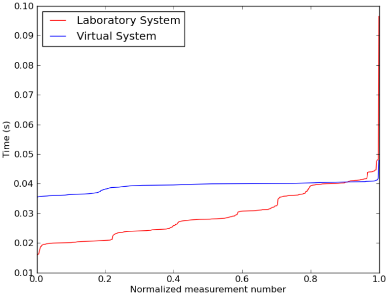
Figure A.1
Master-Slave Interarrival Distribution (Write Command)
138

Figure A.2
Master-Slave Interarrival Distribution (Read Command)
139
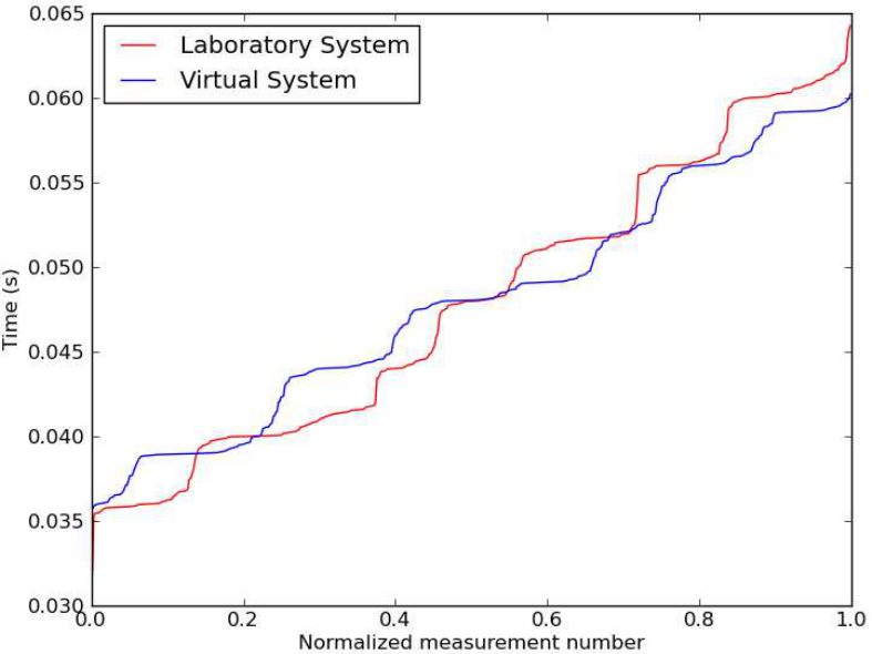
Figure A.3
Master-Slave Interarrival Distribution (Read) After Processing Delay
140

Table A.3
Ground Tank Similarity Scores After Message Processing Delay
Name Similarity Average Error Max. Error Percent Error
Byte Frequency 0.31821 0.00153 0.05530 -0.000%
Byte Throughput 0.95151 -14.83768 -14.83768 10.191%
Error Count 1.00000 - - -
Function Code Count 0.99995 0.00005 0.00042 0.000%
Function Code Sequence 0.99957 - - -
ID Sequence 0.99999 - - -
Interarrival Time 0.91319 0.02239 0.15960 -9.255%
Invalid CRC 1.00000 - - -
Master-Master Interarrival Time 0.91232 0.04218 0.14826 -9.264%
Master-Master Interarrival Time (Read) 0.94973 0.04832 0.12426 -9.213%
Master-Master Interarrival Time (Write) 0.95048 0.04765 0.12407 -9.252%
Master-Slave Interarrival Metric (Read) 0.98309 0.00843 0.02740 0.189%
Master-Slave Interarrival Metric (Write) 0.85697 0.00962 0.03963 26.764%
Master-Slave Interarrival Time 0.92414 0.00492 0.03506 10.619%
Packet Size 0.99998 0.00088 2.00000 -0.005%
Packet Throughput 0.95149 -0.84831 -0.84831 10.197%
Slave-Master Interarrival Metric 0.90222 0.03988 0.15960 -13.146%
Slave-Slave Interarrival Time 0.93182 0.03385 0.15883 -9.252%
the virtual system interarrival times are nearly constant, and roughly 40% of the virtual
master-master interarrival times are greater than the laboratory. In this case, delay should
be added only for the 60% of cases where the error is positive. The additional delay can
be modeled by the piecewise function delay =
0 x < 0.4
0.03265 0.4 ≤ x ≤ 0.835
0.61234 · x x > 0.835
, where x
is a random number from 0 to 1. Table A.4 gives the final resultant similarity scores.
141

Figure A.4
Ground Tank Master-Master Interarrival Time Before Adding Delay
142

Figure A.5
Plot of Interarrival Distribution After Calibration
143

Table A.4
Ground Tank Similarity Scores After Adjusting Master Scan Time
Name Similarity Average Error Max. Error Percent Error
Byte Frequency 0.27601 0.00000 0.01613 -0.000%
Byte Throughput 0.98493 4.32641 4.32641 -2.969%
Error Count 1.00000 - - -
Function Code Count 0.99996 -0.00000 0.00032 0.000%
Function Code Sequence 0.99964 - - -
ID Sequence 0.99995 - - -
Interarrival Time 0.93533 0.00366 0.06616 3.046%
Invalid CRC 1.00000 - - -
Master-Master Interarrival Time 0.94912 0.00731 0.07220 3.038%
Master-Master Interarrival Time (Read) 0.98324 0.01480 0.12166 3.076%
Master-Master Interarrival Time (Write) 0.98385 0.01476 0.11869 3.069%
Master-Slave Interarrival Metric (Read) 0.97891 0.00168 0.02378 3.547%
Master-Slave Interarrival Metric (Write) 0.84308 0.00925 0.02416 31.558%
Master-Slave Interarrival Time 0.91356 0.00548 0.01950 14.420%
Packet Size 0.99999 -0.00083 0.00000 -0.004%
Packet Throughput 0.98495 0.24693 0.24693 -2.966%
Slave-Master Interarrival Metric 0.95694 0.00183 0.08783 0.904%
Slave-Slave Interarrival Time 0.96789 0.00731 0.08484 3.039%
144
