NBER WORKING PAPER SERIES
DIGITAL INFORMATION PROVISION AND BEHAVIOR CHANGE:
LESSONS FROM SIX EXPERIMENTS IN EAST AFRICA
Raissa Fabregas
Michael Kremer
Matthew Lowes
Robert On
Giulia Zane
Working Paper 32048
http://www.nber.org/papers/w32048
NATIONAL BUREAU OF ECONOMIC RESEARCH
1050 Massachusetts Avenue
Cambridge, MA 02138
January 2024
Funding from ATAI, the Dioraphte Foundation, Unorthodox Philanthropy, 3ie, and an
anonymous donor made this study possible. We thank our partner organizations: the Kenya
Agriculture and Livestock Research Organization (KALRO), and in particular to Dr. Martins
Odendo, One Acre Fund (1AF), Precision for Development (PxD), and Innovations for Poverty
Action - Kenya (IPA-K) for all of their support during implementation and data collection. We
are also grateful to 1AF, the Mumias Sugar Company, and German Agro Action
(Welthungerhilfe) for sharing soil data and specially to Dr. Javier Castellanos for generating the
agronomic recommendations to PxD and to Dr. David Guerena for the agronomic
recommendations for 1AF.We thank Lillian Alexander, Carolina Corral, Tomoko Harigaya,
Charles Misiati, Chrispinus Musungu, Cara Myers, Alex Nawar, Carol Nekesa, William Wanjala
Oduor, Violet Omenyo, Victor Perez, and Megan Sheahan for excellent project and research
support. This project benefited from feedback from Rema Hanna, Rohini Pande, Kashi Kafle,
Jessica Zhu, Jack Marshall, Andrew Dustan and participants at AFE, AAEA, MWIDC, the Texas
Experimental Association Symposium, NEUDC, Sao Paulo School of Economics, Development
Inovation Lab, Y-RISE and JILAAE. Disclosure: Michael Kremer is a board member of PxD.
Giulia Zane’s postdoctoral fellowship was funded by PxD. Fabregas, Kremer, and On did not
receive any financial compensation from PxD but the organization partly funded this research. On
worked as a volunteer for 1AF at the time of the experiment. Lowes worked for 1AF. A high-
level summary of the results presented in this paper appears in Fabregas et al. (2019), which cites
a working version of the present article. Experiment registration ID: AEARCTR-0006837. The
views expressed herein are those of the authors and do not necessarily reflect the views of the
National Bureau of Economic Research.
NBER working papers are circulated for discussion and comment purposes. They have not been
peer-reviewed or been subject to the review by the NBER Board of Directors that accompanies
official NBER publications.
© 2024 by Raissa Fabregas, Michael Kremer, Matthew Lowes, Robert On, and Giulia Zane. All
rights reserved. Short sections of text, not to exceed two paragraphs, may be quoted without
explicit permission provided that full credit, including © notice, is given to the source.

Digital Information Provision and Behavior Change: Lessons from Six Experiments in East
Africa
Raissa Fabregas, Michael Kremer, Matthew Lowes, Robert On, and Giulia Zane
NBER Working Paper No. 32048
January 2024
JEL No. Q0
ABSTRACT
Mobile phone-based informational programs are widely used worldwide, though there is little
consensus on how effective they are at changing behavior. We present causal evidence on the
effects of six agricultural information programs delivered through text messages in Kenya and
Rwanda. The programs shared similar objectives but were implemented by three different
organizations and varied in content, design, and target population. With administrative outcome
data for tens of thousands of farmers across all experiments, we are sufficiently powered to detect
small effects in real input purchase choices. Combining the results of all experiments through a
meta-analysis, we find that the odds ratio for following the recommendations is 1.22 (95% CI:
1.16, 1.29). We cannot reject that impacts are similar across experiments and for two different
agricultural inputs. There is little evidence of message fatigue, but the effects diminish over time.
Providing more granular information, supplementing the texts with in-person calls, or varying the
messages’ framing did not significantly increase impacts, but message repetition had modest
positive effects. While the overall effect sizes are small, the low cost of text messages can make
these programs cost-effective.
Raissa Fabregas
The University of Texas at Austin
Michael Kremer
University of Chicago Department
of Economics 1126 E. 59th St.
Chicago, IL 60637
and NBER
Matthew Lowes
One Acre Fund
Robert On
The Agency Fund
Giulia Zane
International Water Management Institute

1 Introduction
The rapid proliferation of mobile phones in developing countries over the past few decades
has opened up new avenues for governments and other organizations to disseminate infor-
mation at scale in pursuit of their policy objectives. As a result, hundreds of digital initiatives
have been deployed to address informational or behavioral barriers and change individual
behavior (GSMA, 2020). While only a fraction of these initiatives have been evaluated, there
is a growing literature assessing the effectiveness of these programs across a range of sectors,
from health (Hall et al., 2014; Jamison et al., 2013), education (Aker et al., 2012; Cunha et al.,
2017; Angrist et al., 2020) and finance (Karlan et al., 2012, 2016) to governance (Dustan et al.,
2018; Buntaine et al., 2018; Grossman et al., 2020) and agriculture (Aker et al., 2016; Fafchamps
and Minten, 2012; Cole and Fernando, 2021).
Much of the empirical evidence on the impacts of these programs on recipient behavior
has been characterized as mixed (Aker et al., 2016; Deichmann et al., 2016; Baum
¨
uller, 2018;
Grossman et al., 2020; Steinhardt et al., 2019). If program effectiveness is very sensitive to
the specific features of its design, the identity of the implementing organization, targeted
recipients, or the local context, it might be difficult to draw broader policy conclusions about
whether to scale up or extend these interventions to a new setting (Pritchett and Sandefur,
2015). However, perceived mixed results could also stem from other methodological issues,
such as sampling variation (Meager, 2019), selection biases (Glewwe et al., 2004), varying
levels of statistical power (Ioannidis et al., 2017), differences in instruments or measurement,
or publication biases (DellaVigna and Linos, 2020).
This paper examines the role of digital interventions on behavior change by presenting
new experimental evidence on the impacts of six text-message-based agricultural extension
programs on individuals’ decisions to acquire recommended inputs. Text messages are inex-
pensive and can reach basic phones without internet connectivity, making them a particularly
attractive option for delivering information in low-income countries where smartphones are
not yet widely adopted.
1
Despite this potential, texting might be too impersonal, light-touch,
or restrictive to meaningfully convey information. Illiteracy, mistrust, or mistargeting might
1
In 2020, we documented that some services in Kenya charged less than $0.006 per text message. In India, it
varied from $0.006 to $0.0004, depending on the number of messages bought. From the point of view of carriers,
the marginal costs of a text message are close to zero.
1

also limit the effectiveness of these types of programs (Aker, 2017), especially when imple-
mented at scale (Bird et al., 2019).
2
The programs examined in this study were implemented in Kenya and Rwanda by three
different organizations: a public agency, a social enterprise, and a research-oriented non-
profit. All the programs shared the goal of increasing farmer experimentation with locally
recommended agricultural inputs. Despite sharing similar objectives and using mobile phones
to reach out to farmers, the programs varied in other dimensions, such as user recruitment
strategies, message content and design, implementation seasons, and complimentary access
to in-person support. This set-up allows us to estimate impacts for each program individually
and aggregate the results through a meta-analysis. The meta-analysis increases statistical
power and enables formal testing for impact heterogeneity across studies. This configuration
also captures a common occurrence in program implementation: organizations with similar
tools and objectives often design and adapt their programs differently based on their specific
constraints, philosophies, and opportunities. When considering scalability, it is important to
understand to what extent these implementation details are critical for effectiveness.
Two features of this study are worth highlighting. First, we present evidence of programs
with substantial sample sizes. In total, over 128,000 individuals participated across all six
experiments. Results from low-powered studies can be mistakenly interpreted as evidence
of no effects if they fail to detect small impacts (Ioannidis et al., 2017; Dahal and Fiala, 2020;
McKenzie and Woodruff, 2014). This interpretation is particularly problematic for very cheap
interventions, such as text messages, since the effect sizes required for these programs to be
cost-effective are usually very small.
2
There is a growing experimental literature on the impacts of text-message-based programs from a variety of
sectors. By far, most empirical evidence comes from evaluations of health programs. Some examples include a
program for adolescent reproductive health messages that found significant effects on knowledge, but no signif-
icant effects on reported intercourse or pregnancy (Rokicki et al., 2017) and positive impacts of SMS reminders
on adherence to antiretroviral treatments (Pop-Eleches et al., 2011). Broader meta-analyses of global text-message
health interventions suggest positive effects on health behaviors (Hall et al., 2015), though the evidence from low
and middle-income countries remains limited (Hall et al., 2014). For financial behaviors in developing countries,
text reminders for microloan repayment were reported to be insignificant unless the message included the loan
officer’s name (Karlan et al., 2015). In a different study, bank clients assigned to receive monthly saving reminders
were three percentage points more likely to meet their commitment (Karlan et al., 2016). The effects of text mes-
sages with moral content reduced credit card delinquency by four percentage points, but researchers did not
find other content to be statistically significant (Bursztyn et al., 2019). In governance, text messages increased
bureaucrat policy compliance by four percentage points (Dustan et al., 2018), and Aker et al. (2017) showed that a
text-message campaign could increase voter turnout. In education, text messages about student truancy increased
school attendance by two percentage points (Cunha et al., 2017). In Peru, Chong et al. (2015) report no statistically
significant effects of text messages on recycling behavior.
2
Second, across all experiments, we use actual input acquisitions as our primary measure
of behavior change. To track the input purchases of farmers affiliated with the social enter-
prise, we use administrative data provided by the organization, as they were directly selling
inputs to farmers. For projects targeting independent farmers, we rely on the redemption of
input discount coupons by both treatment and control farmers in dozens of small agricultural
shops in the region. Using data from real purchasing decisions mitigates the risk that any
estimated effects are driven by social desirability or courtesy bias in self-reports, a common
concern in the evaluation of informational programs (Baum
¨
uller, 2018; Haaland et al., 2020).
Using survey endline data for four programs, we can also compare self-reports against the
administrative records and investigate other outcomes such as knowledge increases and any
potential crowd-out in the use of non-recommended inputs.
Combining the effects of all six programs in a meta-analysis using odds ratios, a relative
measure of effects that is less sensitive to variations in baseline input adoption probabilities,
we find a small but statistically significant effect on following the recommendations (OR:
1.22, 95% CI 1.16 to 1.29, N=6). The aggregate effect for following recommendations about a
newly introduced technology (agricultural lime) is 1.19 (95% CI 1.11 to 1.27, N=6), whereas the
effect for following recommendations for largely unused types of a well-known technology
(chemical fertilizers) is 1.27 (95% CI: 1.15 to 1.40, N=4). With only six studies, we cannot draw
definitive conclusions about the extent of program heterogeneity. However, while we observe
that some individual experiments had statistically significant impacts and others did not, we
cannot reject the hypothesis that the effects were the same and that the observed differences
may primarily stem from sampling variation.
Re-estimating the meta-analysis on the probability of following the recommendations us-
ing an absolute effect measure derived from linear probability models yields a statistically
significant increase of 2 percentage points (95% CI 0.01 to 0.03, N=6). In this instance, we
reject the null hypothesis of homogenous treatment effects across programs. However, the
variation in point estimates across different experiments is small, typically within a range of
one or two percentage points. This observation aligns with the notion that true impact het-
erogeneity across experiments is limited, at least, beyond the variation that can be attributed
to initial levels of input adoption.
While the programs were conceived with the primary intent of providing new information
3
to farmers rather than merely serving as reminders or nudges, the effects seem to operate
partly through behavioral channels. On the one hand, we find positive effects on knowledge.
Treated farmers were significantly more likely to correctly identify the purpose of the newly
introduced input (OR: 1.53, 95% CI 1.38 to 1.70, N=4). On the other hand, the effects on
input purchases waned after one season, but re-treating individuals with the same messages
helped sustain impacts. Moreover, we cannot reject that the impacts on input use were the
same regardless of farmers’ baseline levels of knowledge about these technologies. A potential
interpretation of these results is that well-timed messages might be effective, partly because
they affect how top-of-mind a decision is (Bettinger et al., 2021; Karlan et al., 2015, 2016;
Raifman et al., 2014).
Adding to the literature on behavior measurement (Chuang et al., 2020; Karlan and Zin-
man, 2012) and the work that has found discrepancies between self-reported and actual behav-
ior (Friedman et al., 2015; Karlan and Zinman, 2008), we find significantly larger effects on the
use of the newly introduced input when estimated using survey data compared to adminis-
trative purchase data. While we cannot definitively attribute these differences to survey misre-
porting, within the context of one project, a substantial fraction of farmers for whom there was
a mismatch in the survey and administrative data indicated that they had acquired the input
from sellers who had not stocked it during the same period, according to our monitoring shop
records. This highlights the risk of relying on self-reported data to assess behavior change,
even when the reported behavior is not particularly sensitive. Further, it is difficult to predict
the direction of these inconsistencies; the discrepancy affects some but not all programs, and
we do not identify any significant differences in impacts for the other recommended input.
Finally, we use individual project experimental variation to draw additional lessons about
the importance of different programmatic features. Overall, we do not find strong evidence
that message framing or the specificity of the recommendations make a critical difference.
We cannot reject the hypothesis that messages crafted using behavioral insights (e.g., sense
of urgency, self-efficacy, social comparisons, etc.) were as effective as a basic message. We
also do not detect additional gains from sending messages with more detailed information,
such as highlighting that the recommendations were based on local soil data. The absence of
additional gains in input adoption resulting from providing more specific recommendations
aligns with experimental findings from other contexts (Beg et al., 2024; Corral et al., 2020).
4

To test whether in-person communication could help farmers make sense of the new in-
formation and strengthen its effects, one experiment complemented the text messages by ran-
domizing a phone call from an extension officer. We find no evidence of additional statistically
significant impacts from this add-on. Message repetition, however, was modestly effective at
increasing purchases.
3
We also estimate spillovers for the programs that targeted users who
belonged to farmer groups, and find some suggestive evidence of positive externalities.
Without data on yields, we cannot draw firm conclusions on the effects of these programs
on farmers’ profits.
4
However, using agronomic estimates of the impacts of the recommended
inputs on maize yields, we provide a back-of-the-envelope calculation of the potential direct
benefits of sending these text messages. Our estimates suggest that the benefit-cost ratio of
sending these messages at scale is about 46 to 1. Under these metrics, text messages compare
favorably to more intensive, but also more expensive, programs such as in-person farmer
events.
This paper adds to the recent literature that finds modest but positive effects of low-touch
interventions on behavior change (Benartzi et al., 2017; Oreopoulos and Petronijevic, 2019;
DellaVigna and Linos, 2020). In this case, however, the focus is on digital informational inter-
ventions in low-income contexts. Our results also speak to the literature concerned with the
use of experimental evidence for policy scale-up, particularly in development projects, where
heterogeneity in treatment effects has been used as a measure of external validity (Pritchett
and Sandefur, 2015; Allcott, 2015; Meager, 2019; Vivalt, 2016). We find little evidence to sup-
port the notion that true program impacts are highly heterogeneous, and we suggest caution
in qualitatively interpreting differences in statistical significance across studies because these
differences could be driven by sampling variation and studies underpowered to detect small
effects.
Finally, we complement expert qualitative summaries of the literature on digital interven-
tions for development (Aker, 2017; Aker et al., 2016) and the handful of experimental studies
3
The sample sizes used in the experiments on message repetition were much larger than those in the in-person
call and better powered to detect small impacts. However, given that the costs of in-person calling are much
higher, it is unlikely that this approach would be cost-effective at the estimated effect magnitudes.
4
Measuring impacts on downstream outcomes, such as yields and profits, can be complex if the effect sizes that
would make these types of programs cost-effective are small. Self-reported yields are noisy (Lobell et al., 2018),
and objective measures such as physically harvesting a section of a farmer’s plot could be prohibitively expensive
to gather at the required sample sizes. The stochastic nature of rainfall and other features can further complicate
this (Rosenzweig and Udry, 2020).
5

assessing the impacts of digital agricultural extension systems. Larochelle et al. (2019) study
a text-based program for potato farmers in Ecuador and found that the program increased
knowledge and self-reported adoption of integrated soil management practices. Text mes-
sages sent by an agribusiness to sugar cane farmers in Kenya had positive yield impacts in
one trial but no significant effects in a second trial (Casaburi et al., 2014). Fafchamps and
Minten (2012) report null effects from a text-based program with weather, price, and advisory
content in India. A more sophisticated voice-based service, targeted at cotton farmers in India,
increased the use of recommended seeds but no other inputs (Cole and Fernando, 2021). This
paper expands what is known empirically about text-based agricultural extension programs,
addressing some methodological limitations in existing work.
5
This paper is organized as follows: section 2 presents the context and design of each pro-
gram and their evaluations. Section 3 discusses the empirical strategy. Section 4 provides the
main results, and section 5 discusses some of the additional lessons that we can be drawn from
individual experiments. We present cost-effectiveness estimates in section 6 and conclude in
section 7.
2 Context, Programs and Experimental Design
2.1 Context
The programs targeted maize smallholder farmers in Rwanda and Kenya between 2015 and
2019 (see Appendix Figure A1 for a map).
6
In both countries, maize is farmed twice a year. In
Kenya, the primary agricultural season, the long rain season, runs from March until August,
and a secondary agricultural season, the short rains season, from September to December.
The main season in Rwanda is from September to January, and the secondary season is from
5
A couple of additional literatures are worth highlighting here. First, the literature on the broader effects of
mobile phone access on market performance and productivity (Jensen, 2007; Gupta et al., 2020; Aker and Mbiti,
2010; Aker and Fafchamps, 2015). Second, the studies on the market effects of providing information about crop
prices through mobile phones (Camacho and Conover, 2010; Mitra et al., 2017; Nakasone et al., 2014; Courtois
and Subervie, 2014; Svensson and Yanagizawa, 2009). Finally, other digital extension approaches, like delivering
information via video, tablets, or smartphone apps, have also been shown to have positive effects on farmers’
beliefs and behaviors (Tjernstr
¨
om et al., 2019; Van Campenhout et al., 2020; Arouna et al., 2019). However, until
smartphone penetration increases, such approaches will likely require an in-person or third-party component to
deliver them to the average farmer.
6
The adult literacy rate in Kenya is 82% and in Rwanda is 73% (UNESCO, 2022). Estimates of mobile phone
penetration in 2017 were 87% for Kenya and 48% in Rwanda, though significant urban-rural gaps exist (Gillwald
and Mothobi, 2019).
6

March to August.
In these areas, maize is a staple food and traded commodity, and increasing smallholder
productivity is an important policy objective to improve food security and reduce poverty.
However, smallholder yields have remained low, partly due to soil degradation, soil acidity,
and the low adoption of productivity-enhancing technologies (FAO, 2015).
High soil acidity can dramatically reduce crop yields by limiting nutrient availability to
plants (The et al., 2006; Tisdale et al., 1990; Brady and Weil, 2004). Optimal pH for crop
growth is around 6.0-7.0. Soil pH under 5.5 is considered strongly acidic, and it is a standard
pH threshold under which the soil is deemed unsuitable for maize growth (Cranados et al.,
1993; Kanyanjua et al., 2002). The application of agricultural lime to the soil is one of the
cheapest and most widely recommended methods to increase soil pH. Several public agencies
and NGOs in Africa have advocated for the use of lime, and experimental plots conducted
in Kenya suggest that lime application can increase maize yields by 5-75% depending on the
area, soil characteristics, rate applied, etc. (Kisinyo et al., 2015; Gudu et al., 2005; 1AF, 2014).
Yet agricultural lime is not a widely known or used input. In Kenya, only 7% to 12% of
farmers in our samples reported having ever used it at baseline, and in Rwanda, only 6% had
purchased it during the previous season.
Chemical fertilizers are more widely used, but most farmers in the sample areas have only
used a specific type of phosphate-based fertilizer, diammonium phosphate (DAP), applied at
planting time. Few farmers regularly experiment with other options, such as top-dressing
fertilizers like calcium ammonium nitrate (CAN) and urea, which are applied to the plant
once it has started to mature.
7
Fertilizers, particularly top-dressing ones, can be profitable
(Duflo et al., 2008; Kelly and Murekezi, 2000) and current national and international recom-
mendations have started to encourage farmers to use fertilizers that best fit their soil and local
conditions (KSHC, 2014; NAAIAP, 2014). Therefore, several organizations have also attempted
to inform farmers about different fertilizer options to encourage experimentation.
One potential reason for the low uptake and/or experimentation with locally suitable tech-
nologies is that many smallholders lack reliable access to science-based agricultural advice.
7
In Kenya, over 80% of farmers in our sample reported using planting fertilizers in the previous seasons. This
proportion is higher than that reported in other contexts in the region (Sheahan and Barrett, 2017). Indeed, input
use in Kenya is also much higher than in neighboring countries. In 2019, the FAO estimated that Kenya’s average
nitrogen fertilizer use was 22kg, which is similar to that of Ethiopia (23 kg) but higher than that of Uganda (1.2
kg), Tanzania (9 kg), or Rwanda (7 kg).
7

Access to extension services is rare for farmers not engaged in agricultural programs pro-
moted by NGOs or other organizations. Acquiring information about locally relevant inputs
is not trivial, even if farmers find this advice valuable (Fabregas, 2019). For instance, there can
be significant frictions in information sharing among peers (Chandrasekhar et al., 2022), and
learning through self-directed experimentation can be difficult if farmers do not know pre-
cisely along what dimensions to experiment (Hanna et al., 2014) or if they misperceive their
soil characteristics (Berazneva et al., 2016). Moreover, potential heterogeneity in soil character-
istics and the profitability of inputs (Marenya and Barrett, 2009; Suri, 2011) makes it difficult
to rely on national or regional-level blanket recommendations.
Knowledge gaps are apparent in the data. For example, in the initial program evaluation in
Kenya, at baseline, 66% of farmers considered soil acidity to be a significant issue for their soil.
However, among these, 44% were unaware of any methods to address this problem, and only
15% were familiar with agricultural lime as a potential solution. Combining all samples for
which we have data on farmers’ knowledge, we estimate that only 32% of untreated farmers
were able to recognize lime as a potential solution to high soil acidity.
2.2 Partner Organizations, Programs, and Randomization
This section briefly summarizes the characteristics of the implementing organizations, their
programs, and the main features of each evaluation.
8
The common treatment across all pro-
grams was information provision about agricultural lime. Four programs also sent informa-
tion about locally recommended chemical fertilizers. Table 1 summarizes the six programs,
and Table 2 briefly describes the characteristics of each experiment. Further details about each
program and evaluation are discussed in Appendix J.
2.2.1 KALRO
The Kenya Agriculture and Livestock Research Organization (KALRO) is a Kenyan semi-
autonomous public agency with the mandate to promote agricultural research and dissemina-
tion. KALRO’s text-message program was developed in partnership with the Kenyan Ministry
of Agriculture and was envisioned as a low-cost way to reach farmers with simple messages
8
We define an ‘implementing organization’ as the primary organization in charge of designing the programs,
crafting the messages, and delivering them. Each implementing organization faced its own constraints, goals, and
directives. IPA and PxD-affiliated researchers were involved in analyzing and evaluating all six programs.
8

9
Table 1: Program Characteristics
KALRO IPA/PxD1-K IPA/PxD2-K 1AF1-K 1AF2-K 1AF3-R
(1) (2) (3) (4) (5) (6)
Org. KALRO IPA/PxD IPA/PxD 1AF 1AF 1AF
Org. Type Public NGOs NGOs Social Enter-
prise
Social Enter-
prise
Social Enter-
prise
Location Kakamega and
Siaya (Kenya)
Busia and
Kakamega
(Kenya)
Busia,
Bungoma,
Kakamega &
Siaya (Kenya)
Busia and
Kakamega
(Kenya)
Bungoma, Bu-
sia, Kakamega
and Vihiga
(Kenya)
Western, East-
ern, Southern
(Rwanda)
Agricultural
Season
SR 2015 SR 2016/LR
2017
LR 2017 LR 2017/LR
2018
LR 2018 Main Season
2017/2018
Recruitment Farmers
drawn from
village census
survey
Former NGO
and contract
farming par-
ticipants
Clients of
agrodealers
1AF clients in
LR 2016
1AF clients in
LR 2017
1AF clients in
2016
Eligibility Farmed dur-
ing past year,
in charge of
farming
Planted maize
in 2016, reside
in program
area
Clients of
agrodealers
1AF clients in
LR 2016
1AF clients in
LR 2017
1AF clients in
2017
Message Con-
tent
Lime, fertil-
izer, seeds,
field manage-
ment
Lime, fer-
tilizer, field
management
Lime and fer-
tilizer
Lime Lime and fer-
tilizer
Lime
Number of
Messages
21 total (2
acidity/lime; 3
fertilizer)
24-28 total (7-
9 acidity/lime;
4-9 fertilizer)
13 total (6
acidity/lime; 4
fertilizer)
6 total (6 acid-
ity/lime; 0 fer-
tilizer)
1-10 total (1-
5 acidity/lime;
1-5 fertilizer)
1-4 total (1-4
acidity/lime; 0
fertilizer)
Timing Throughout
season
Throughout
season
Before plant-
ing and top-
dressing
Before input
choice
Before input
choices
Before input
choice
Lime recom-
mended?
All (if acidic) 0.81 0.76 All All All
Key Fertil-
izers recom-
mended
DAP, NPK,
CAN, Mavuno
Urea Urea - CAN -
Used Local
Soil Data?
No Yes Yes Yes Yes Yes
Additional
Services?
No No Phone-call 1AF Services
& Call-center
1AF Services
& Call-center
1AF Services
& Call-center
Any Message
Repetition
No Yes Yes Yes Yes Yes
Opt-in 1 0.95 0.95 - - -
Previous lime
use
b
0.07 0.12 0.09 - - 0.06
Previous sea-
son fert. use
(any/recommended)
b
0.84/0.84 0.92/0.18 0.88/0.19 0.95/- 0.93/0.15 0.95/-
Female
b
0.65 0.37 0.34 0.64 0.69 -
Primary
School
b
0.53 0.60 0.72 - - -
Notes: SR denotes Short Rain Season and LR Long Rain Season.
b
denotes data for the control group at baseline. - denotes that
data is unavailable. Lime recommended indicates whether all farmers received messages recommending positive amounts of lime or the frac-
tion that did. Key fertilizer recommended whether fertilizer messages were sent, and if yes, the types of fertilizer. Opt-in indicates the frac-
tion of farmers who, when invited, agreed to receive texts. A requirement across all programs was to have access to a mobile phone.

to help them adopt locally adapted inputs and practices. A total of 21 agriculture-related mes-
sages were sent throughout the 2015 short rain season. Among these, two messages pertained
to lime usage, while three messages focused on chemical fertilizers. KALRO developed mes-
sages to ensure agronomic accuracy, for instance, advising farmers to use lime if their soil’s
pH was below 5.5. This is in line with the observation that public extension services often
prioritize sending correct agricultural information, but that it may be too technical or not
sufficiently actionable when communicating with the average farmer (Fabregas et al., 2019).
Participating farmers were recruited by field agents who went door-to-door in KALRO’s
catchment areas. Among all identified farmers, 95% met the inclusion criteria for the study
(i.e., phone owner, responsible for farming, and had planted maize during the previous sea-
son) and were invited to complete a baseline survey. Farmers were then randomized at the
individual level into a treatment or a control arm.
9
All farmers invited to participate in the text
message program opted in. The baseline sample consisted of 832 farmers, of which 733 later
completed an endline survey. From these, about two-thirds were females, and before treat-
ments started, only 7% reported ever using lime, whereas 84% had used chemical fertilizers
during the previous season (Appendix Table C1).
2.2.2 IPA and PxD
Innovations for Poverty Action (IPA) is a research and policy organization, and Precision
for Development (PxD) is a non-profit organization that supports the provision of phone-
based information services to smallholder farmers in developing countries. We discuss the
evaluation of two programs, IPA/PxD1-K and IPA/PxD2-K, implemented in Kenya through
a partnership between these two organizations.
Ensuring that messages provided actionable guidance for farmers was a central objective
of the IPA/PxD projects. Recognizing that few smallholder farmers would conduct individual
soil tests on their farms due to their relatively high cost and limited availability, the programs
used information from area-level soil tests to provide recommendations (Appendix K de-
scribes soil data sources and how recommendations were built). Based on these soil samples,
81% of the sample in IPA/PxD1-K and 76% in IPA/PxD2-K were recommended to experiment
9
As part of this project, a second treatment arm, testing in-person farmer field days, was also evaluated. The
results are described in Fabregas et al. (2017b).
10
with lime in a small area of their land.
Another factor to consider is that while agricultural lime is cheap, it is bulky. Farmers often
find it challenging to transport and store it in sufficient quantities for widespread application.
As a solution, farmers were advised to opt for micro-dosing, targeting the base of the plants.
This approach entails a lower dosage but requires re-application each season. In experimental
plots, lime micro-dosing increased yields by up to 14% (1AF, 2014).
(i) IPA/PxD1-K. The first text message program was implemented during the 2016 short-rain
agricultural season. Participants were identified using existing regional farmer databases.
A sample of 1,897 farmers completed a short baseline survey over the phone and was later
randomized into two treatment arms or a control arm. Farmers in the first treatment arm
(General SMS) received messages with general agricultural advice. These messages mentioned
the purpose of lime and recommended using fertilizers, but did not reference the soil test data.
The messages received by farmers in the second arm (Specific SMS) referred to the area-level
soil data and contained more precise details, such as additional guidance on recommended
input quantities. Among those randomized into the treatment groups, 95% agreed to receive
the messages. Depending on the intervention arm, between 24 and 28 messages were sent,
each text timed to the moment in which it would be most relevant. Of these, 7 to 9 messages
dealt with soil acidity and lime, 4 to 9 were about fertilizers and the rest covered topics related
to other management practices.
During the following agricultural season, the 2017 long rains, both treatment arms received
five identical messages promoting the use of agricultural lime (for areas where lime was
recommended). The control group remained untreated.
The sample for this experiment was 37% female. At baseline, only 18% had used one of the
key recommended fertilizers in the previous season, and approximately 12% had ever used
lime (Appendix Table C2).
(ii) IPA/PxD2-K. During the long rain season of 2017, a second text-message program was
implemented by IPA/PxD, targeting a different sample of farmers and expanding its reach
to include two additional areas. This program sent 13 messages solely focused on lime and
fertilizers. Messages were sent right before the time for planting or top-dressing. Farmer
recruitment was done via agricultural supply dealers (agrodealers or agrovets) who invited
11

existing clients to register to participate.
10
Once registered by the agrodealer, a member of the research team contacted farmers via
phone to obtain consent to participate in the study and complete a brief baseline survey.
Farmers were randomly assigned to one of three treatment arms or a control group following
this survey. The first arm received only text messages (SMS only). The other arms were
designed to investigate whether real-time communication with a person could strengthen the
texts. Therefore, in the second arm, farmers received a phone call from an extension officer
(SMS + Call), while in the third arm, farmers could request to receive a call (SMS + Call Offer).
The final sample consisted of 5,890 farmers, of which 34% were female, 9% had used lime in
the past, and 19% had used the key recommended fertilizer (Appendix Table C3).
2.2.3 1AF
One Acre Fund (1AF) is a social enterprise operating across six countries in Eastern and
Southern Africa. 1AF’s model relies on training farmers in modern agricultural techniques
and providing them with inputs on credit early in the agricultural season, which they later
repay. 1AF clients form groups of eight to eleven farmers who participate in the program
together and are supported by a local 1AF field officer.
To address the problem of high soil acidity, 1AF offers farmers agricultural lime as an
optional input. However, demand for lime was relatively low across their operating locations.
Hypothesizing that this low demand could reflect a lack of awareness, 1AF implemented two
text-message programs in Kenya and one in Rwanda to encourage lime use (1AF1-K, 1AF2-
K, and 1AF3-R).
11
Messages were sent before and during 1AF ‘enrollment season’, that is,
the period in which farmers register for the 1AF program and make input orders. To build
area-level acidity recommendations, 1AF used its own soil data (see Appendix K).
12
(i) 1AF1-K. 1AF’s first text-message program was implemented in western Kenya. During the
10
This method offered several advantages. First, it was a low-cost and quick method to recruit farmers. Second,
farmers who are clients of agricultural supply dealers might already be more likely to acquire inputs, be less
credit-constrained, and therefore be more likely to benefit from an information-based program.
11
Relative to farmers in other samples who rarely had contact with extension officers, 1AF farmers receive
intensive agricultural extension training. One goal of using a digital approach, however, was to devise a cheap
way to convey new information that did not require additional training and delivery by 1AF field officers, who
already followed detailed and lengthy farmer training protocols.
12
In addition, all of their programs offered a hotline to treated farmers. Farmers could call if they had more
questions about lime. Take-up of this hotline was extremely low, with less than 1% of farmers using this service.
12
2017-long rain season, the program sent six messages about lime. Farmers were randomized
into either of two treatment arms or a control. The first arm sent simple text messages alerting
the recipients about soil acidity and encouraging them to use lime (Broad SMS). A second
group received more detailed messages that mentioned the predicted level of acidity in the
area, the amount of lime recommended and the expected returns to its application (Detailed
SMS). Participants were randomly selected from lists of previous 1AF clients in Busia and
Kakamega counties. A final sample of 4,884 farmers participated in the experiment.
For the following 2018 long rain season, farmers from the previously mentioned sample
who had participated in the 1AF program in 2017 were re-randomized into treatment and
control. Those in the treatment group received messages promoting lime adoption. A total of
2,931 farmers were re-randomized into receiving messages, allowing us to measure outcomes
for three groups: farmers who were never assigned to receive messages, farmers who received
messages during two consecutive long rain seasons, and farmers who were only treated dur-
ing the first season but not the second one.
(ii) 1AF2-K. A second program was implemented in the Kenyan counties of Bungoma, Busia,
Kakamega and Vihiga during the 2018 long rain season. A total of 32,572 farmers participated
in this experiment, all of them recruited through prior 1AF clients listings. Farmers were
randomized at the individual level into a comparison group or one of two treatment arms: a
Lime only group, which received messages only concerning lime, and a Lime + CAN group,
which received messages about lime and the top-dressing fertilizer CAN. The larger sample
size made it possible to cross-randomize message framings and repetitions (1 to 5 messages)
among treated farmers. The different framing versions included a basic message and messages
that highlighted yield increases, encouraged experimentation, made social comparisons, and
promoted self-efficacy. Moreover, the message content was cross-randomized to send mes-
sages addressing the whole family instead of the individual. During the second agricultural
season, 1AF sent lime-related messages to both control and treated farmers, effectively ending
the lime experiment but allowing us to study the persistence of effects on fertilizer use.
(iii) 1AF3-R. The third 1AF program was first implemented across Rwanda in 2017. This
program consisted of sending only lime-related text messages. The experiment was designed
as a two-staged randomized experiment, which enabled the identification of spillover effects.
Farmer groups were randomly assigned to one of three arms: the full control arm (Full Con-
13
trol), where no farmers received messages; the fully treated arm (Full Treatment), where all
farmers with phones received messages; and the partially treated arm (Partial Treatment),
where farmers with phones were further randomized into either receiving messages or re-
maining as controls. This design allows studying the extent of spillovers by comparing the
outcomes of untargeted farmers in partially treated groups against those of farmers in the full
control group. Furthermore, one can also estimate spillovers on individuals who do not own
mobile phones by comparing non-phone owners in both treatment and control groups.
The sample included 20,944 farmer groups, comprising 202,972 farmers. To study the
direct effects of the program, we focus on the sample of 82,873 farmers who, at baseline, had
phones and were not assigned to the control condition in the partially treated groups.
Like 1AF2-K, message framings and repetition were randomized among treated farmers.
The different framing versions included a simple general message and messages that high-
lighted yield impacts, encouraged self-diagnosis, referred to the use of soil data, explained
how lime works, encouraged farmers to order immediately, highlighted soil acidity and im-
pact issues, and emphasized yield changes. The messages were further cross-randomized to
be framed as a loss or a gain.
The following agricultural season, groups were re-assigned to treatment or control (only
those who had enrolled in the 1AF program in 2018 were eligible to be re-randomized). In-
dividual farmers within treated groups were further randomized to receive or not receive
messages. This created random variation to study the impact of messages over one or two
seasons.
2.3 Considering Heterogeneity in Lime Requirements
Mobile phones offer a unique advantage over other mass distribution channels like radio
or television in that they allow for personalized communications. This proved important in
delivering information about agricultural lime, which is only recommended for acidic soils.
IPA/PxD and 1AF capitalized on this advantage by sending messages based on area-level soil
pH information rather than providing blanket recommendations at the district or province
level. The goal was to improve upon the status quo, in which farmers receive either no
information or very generic advice.
Despite this attempt to provide more accurate information, the impacts of using lime
14

Table 2: Research Design
KALRO IPA/PxD1-K IPA/PxD2-K 1AF1-K 1AF2-K 1AF3-K
(1) (2) (3) (4) (5) (6)
Unit of ran-
domization
Individual Individual Individual Individual Individual Cluster
(farmer group)
Sample Size 773 1,897 5,890 4,884 32,572 82,873 (27,527
groups)
Treatment
Arms (#)
1 2 3 2 2+ 2+
Treatment
Arms
1.SMS 1.General
SMS, 2.Spe-
cific SMS:
sent additional
information
about local
acidity level,
input prices
and quantities.
1.SMS only,
2.SMS + Call:
also received
call by field
officer, 3.SMS
+ Call offer:
also offered to
receive phone
call
1.Broad SMS,
2.Detailed
SMS: addi-
tional info on
degree of soil
acidity, lime
quantity, cost,
and predicted
yield increase.
1.Lime only,
2.Lime +
CAN: ad-
ditional
messages
encouraging
to buy extra
CAN. Cross-
randomized:
message
framing and
repetitions.
1.Full treat-
ment: all
farmers in
a group got
SMS. 2.Partial
treatment:
half farmers
in group got
SMS. Cross-
randomized:
message
framing and
repetitions.
Second Sea-
son SMS
No Yes, maintain
treatment sta-
tus
No Yes, cross-
randomized
Yes, all Yes, cross-
randomized
Admin Out-
come
Coupon (pa-
per), LR 2016
Coupon (digi-
tal), SR 2016 &
LR 2017
Coupon (digi-
tal), LR 2017
1AF admin,
LR2017 &
LR2018
1AF admin,
LR2018 &
LR2019
1AF admin,
2017 & 2018
Coupon Value 50% discount
lime, 50% dis-
count td fertil-
izer
Choice 10 Kg
lime or soap
(first season);
15% discount
lime (second
season); 30%
discount CAN
or urea
15% discount
lime; 15% dis-
count fertilizer
- - -
Baseline Sur-
vey
Yes Yes (phone) Yes (phone) No No No
Endline Sur-
vey
Yes, SR 2015 Yes (phone),
LR 2017
Yes (phone),
LR 2017/SR
2017
Yes (phone),
LR 2017
No No
Note: All experiments included a control group in addition to the treatment arms. SR and LR denote the Short and the Long Rain
agricultural season in Kenya, respectively. Topdressing is denoted as td. Treatment arms (#) denotes the number of treatment
arms, for 1AF ‘+’ indicates that there were cross-randomizations in these samples for the number of messages (1-5), and framing.
ultimately depend on the soil needs of each individual farm. For example, some farmers in
areas deemed acidic may have received messages suggesting they experiment with lime even
if their own soil was not acidic.
To better understand the extent of heterogeneity in soil acidity within the treated areas,
15
we analyze data from over 9,000 soil tests conducted in the areas of study. To the extent that
the farms where these soil tests were conducted are representative of the land of participating
farmers, this gives a rough sense of the share of farmers in treated areas who would have
experienced agricultural gains from lime use. A naive estimate of this share suggests that
within areas where lime was recommended, 90% of tests were below a pH of 6.0 in areas
where lime was recommended (68% below a pH of 5.5 and almost all below a pH of 7)
(Table K1, columns (2)-(4)). However, soil measurements are subject to many sources of error.
For instance, the test-retest correlation of pH was 0.7 in a subset of soil samples blindly tested
twice by the soil laboratory. Adjusting our estimates for this type of measurement error, we
predict that over 97% of soil samples within recommended areas fell below the pH threshold
of 6 (see Appendix K for details).
In practice, based on data from 1AF’s lime experimental plots for which soil test data also
exists, we cannot reject that the effects of lime on maize yields were the same on farms where
soil pH tested below or above 5.5 (Appendix Figure K2). This also suggests that relying on
‘hard’ soil acidity cutoffs using a single soil test for a plot of land might be too restrictive.
We also consider the differential costs that farmers in the treatment group may have faced
when experimenting with lime. Firstly, the potential for overliming and causing soil alka-
linity was minimal at the recommended levels (see Appendix K). Therefore, the main costs
would have been related to the time and money spent on acquiring and applying the input.
Fortunately, lime is very cheap. At the average amounts of lime used between treatment and
control, we estimate that the differential expenditure on lime purchases was less than a dollar,
even when conditioning on purchasing a positive amount of lime. Thus, even if some farmers
might not have realized yield benefits from applying lime, the incurred costs seem reasonable
in relation to the benefits gained from learning about the effectiveness of this input on their
soil, particularly in a context where individual soil tests are very expensive for the average
farmer ($15-20).
Finally, we note that each organization was aware of these issues and consequently encour-
aged farmers to experiment or seek more information before making substantial investments
in lime. IPA/PxD advised farmers to always start by experimenting in a small area of their
farm and only then scale. KALRO urged farmers to test their soils individually before us-
ing lime. 1AF relied on its extensive in-person extension network to provide farmers with
16
additional support as necessary.
2.4 Data
2.4.1 Baseline Data
An in-person baseline survey data was collected for the KALRO sample before the randomiza-
tion took place. A phone-based baseline survey was completed with farmers in the IPA/PxD1-
K and IPA/PxD2-K programs. All these surveys asked about demographics, prior agricultural
practices, and input use. For the 1AF projects, we rely on client administrative data from the
previous seasons, which reported gender and previous input purchases from 1AF.
2.4.2 Endline Data
Endline survey data for farmers was collected for the KALRO, IPA/PxD1-K, IPA/PxD2-K,
and 1AF1-K programs. Additionally, there is at least one administrative measure of real input
acquisitions for each program. For KALRO and IPA/PxD, we use data from coupons that
treatment and control farmers could redeem at local agrodealers. The coupons were devised
as a way to observe real input choices while minimizing experimenter demand effects. To
ensure that people would bring in the coupons when acquiring inputs, they were tied to price
discounts that varied by project. While any discounts should have affected treatment and
control group farmers in similar ways, this implies that we observe demand at prices that
would not have existed in the absence of these programs. For the 1AF projects, our primary
measure of input choice consists of farmers’ agricultural input orders placed with 1AF.
Considering the diverse characteristics across the program contexts we investigate — rang-
ing from the extent of farmers’ liquidity constraints and area-level cellphone signal strength to
local maize prices and regional availability of agricultural supply dealers, we take the hetero-
geneity in input prices faced by farmers as an additional source of variation across projects.
KALRO. At the end of the 2015 agricultural short rain season, farmers in the KALRO sam-
ple were visited and asked to complete an in-person endline survey. The survey contained
knowledge and input use modules. During this visit, all treatment and control group farm-
ers received two paper coupons redeemable for inputs at a discount at selected agricultural
supply dealers in their nearest market center. The first discount coupon was redeemable for
17
a 50% discount for agricultural lime. The second coupon was redeemable for a 50% discount
for any chemical fertilizer of their choice (CAN, DAP, NPK, or Mavuno). All coupons had a
unique ID that allowed us to link redemption to respondents. Participating agrodealers were
asked to keep the coupons and record farmers’ input choices and purchases. For the KALRO
sample, the survey measures behavior changes concurrent with the program implementation,
whereas the coupons measure input purchases for the subsequent agricultural season.
IPA/PxD. The IPA/PxD-managed programs sent input discount coupons via text message
to all treatment and control farmers in their respective samples early in the season. Farmers
could redeem the coupons with agrodealers in their preferred market center (reported at
baseline). For the IPA/PxD1-K program, both lime and fertilizer coupons were sent during
the 2016 short rains. The lime coupon was redeemable for either 10 kg of lime or 1 bar
of soap. Allowing farmers to choose between lime and another commonly used product
of similar value was done to capture farmers’ input choices without liquidity constraints.
The second coupon provided a 30% discount on any top-dressing fertilizer (mavuno, urea or
CAN). For the subsequent agricultural season, the 2017 long rain season, all farmers received
lime coupons for a 15% discount. During this program, 32 agrodealers in 25 distinct market
centers participated in coupon redemption. A phone endline survey was conducted during
the 2017 long rain season with this sample. The survey included questions about input use
during the 2016 short rains and 2017 long rains.
The sample of farmers participating in the IPA/PxD2-K program received one electronic
coupon redeemable for a 15% discount for lime and another one for a top-dressing fertilizer
of their choice. These coupons were only sent during the long rain 2017 season. For this
program, IPA/PxD partnered with 102 agrodealers in 46 market centers. A phone endline
was also completed with this sample, in which the exact timing of data collection (end of long
rain or subsequent short rain) was randomized.
1AF. Outcomes for all 1AF programs were measured through the agricultural input or-
ders placed with the organization. One consideration is that the text-message interventions
occurred before farmers enrolled in the 1AF input program for that particular agricultural sea-
son. Across all 1AF interventions, between 60 and 76% of farmers who received text messages
later enrolled to acquire inputs from 1AF. While we do not find any evidence of differential
1AF enrollment by treatment status (Appendix Table C7, panels D-F, columns (4) and (8)), we
18

take a conservative approach and define our outcome variable as lime purchased through 1AF,
without conditioning on whether farmers were 1AF clients at the time of the experiment.
13
In addition to the administrative data, a random subsample consisting of 30% farmers in
the 1AF-1 sample were invited to complete a phone-based endline survey.
3 Empirical Strategy
3.1 Estimating Individual Program Impacts
Our primary outcomes are ‘following lime’ and ‘following fertilizer’ recommendations. The
indicator variable ‘following lime recommendations’ takes the value of one for farmers in the
treatment and control groups if the farmer used lime and lime was recommended (or would
have been recommended) or if the farmer did not use lime and lime was not recommended
(or would not have been recommended).
14
‘Following fertilizer recommendations’ takes the
value of one if farmers purchased at least one of the key recommended fertilizers for which
administrative data is available and set to zero otherwise (recommended fertilizers are listed
in Table 1). For programs for which we have access to survey data, we can also measure
changes in agricultural knowledge and use of other inputs.
In all cases, we estimate intention-to-treat (ITT) effects.
15
The general equation we estimate
13
This will tend to underestimate impacts since farmers who did not re-enroll in the 1AF program would not
have been able to buy inputs from the organization. We also report effects in the Appendix, restricting the sample
of farmers to those who re-enrolled during the season of the text-message program (Table D2, columns (5), (6),
(11), and (12)). To study effect persistence, we also estimate differential 1AF enrollment by treatment status over
a second season and do not find statistically significant differences (Appendix Table C7, panels D-F, columns (5)
and (9)).
14
The 1AF programs recommended positive amounts of lime to all farmers. KALRO recommended farmers to
test their soil and use lime if their soil was acidic. Since the program took place in an acidic region, we assume
purchasing lime is equivalent to following lime recommendations for this sample.
15
Some farmers might not have received or read the messages. Unfortunately, the technology used to text
farmers does not make it possible to determine whether the messages were opened. Using survey data, we
document the following fraction of farmers who reported receiving agricultural information via text at endline:
54% in the 1AF1-K trial, 67% in the KALRO trial, 81% in the IPA/PxD2-K trial, and 92% in the IPA/PxD1-K trial.
These differences could be explained by a variety of factors, including cellphone signal reception, the share of
incorrect numbers held by each organization, the amount of time between receiving messages and completing
the survey, and the way in which questions were asked. Since there is uncertainty around how precise these
self-reports are, we report effects as intention-to-treat rather than attempting to scale them. This strategy will
underestimate the impact of receiving the messages. However, it will more adequately address the policy question
of the effects of these types of programs, knowing that not all recipients will engage with the messages.
19
for each program is:
y
i
= α + βTreatment
i
+ γ
k
+ e
i
, (1)
where y
i
is the outcome measure for farmer i. Treatment
i
denotes a dummy variable(s) indi-
cating treatment, γ
k
is a vector of randomization strata (if used in the specific experiment), and
e
i
is the error term. The estimated coefficient β denotes the difference between treatment and
control farmers. Since several experiments tested several treatment arms and message vari-
ants, our main results show estimates pooling all treatment arms together to increase power
and simplify the analysis and discussion. However, we provide tables with results for each
treatment arm in Appendix F and highlight some lessons from these experimental variations
in Section 5.
For binary outcomes, we estimate linear probability models and non-linear analogs to
equation 1 using a logistic regression model and reporting the coefficient β in terms of odds
ratios (OR). This modeling choice reflects a concern to select an appropriate summary measure
for a metanalysis, as discussed further below.
Our main specifications only control for the strata used in each randomization, as applica-
ble. As an additional robustness check, the Appendix presents results where we incorporate
controls for other farmer demographic characteristics, baseline farming practices (as avail-
able), and location-fixed effects. In the case of survey data, we also include enumerator-fixed
effects. Appendix B contains a list of strata and additional controls used for each project.
For randomizations at the individual level, we do not cluster standard errors. For the
1AF3-R experiment, error terms are clustered at the farmer group level (the level of random-
ization).
3.1.1 Validity of the Experimental Designs
Appendix Tables C1-C6 show baseline characteristics by treatment status together with tests
of equality of means across treatment arms for each program. As expected, the treatment and
control arms are balanced along most characteristics. While some differences are statistically
significant, most F-tests of joint orthogonality for baseline variables that use specifications
that include stratification variables fail to reject the null that coefficients are jointly zero for all
20

experiments.
16
Out of attempted surveys, the survey completion rate ranged from 79% (IPA/PxD1-K and
1AF1-K) to 92% (KALRO). To investigate the potential for differential attrition, we regress
survey attrition dummies on treatment indicators. We do not find any evidence of differential
attrition by treatment status for any of the projects that collected endline survey data (Ap-
pendix Table C7, panels A-D, columns (1) and (6)). In the IPA/PxD and the 1AF1-K endline
surveys, certain questions regarding lime use and knowledge were only asked to those who
had planted maize during the 2017 long rain season (97%, 98% and 94% of those who com-
pleted the IPA/PxD1-K, IPA/PxD2-K and 1AF1-K surveys, respectively). To keep samples
consistent across various outcomes, we condition all outcomes on maize cultivation during
that season. Importantly, there are no differences in the probability of having differential
missing data by treatment status with this additional condition (columns (2) and (7) in pan-
els B-D). As previously discussed, for 1AF programs, we find no differential likelihood of
re-enrolling in subsequent 1AF program seasons due to the treatment (columns (3)-(5) and
(8)-(10) in panels D-F).
3.2 Meta-analysis
To synthesize the evidence across these various experiments and present a weighted average
of the study estimates, we combine the results in a meta-analysis. We use a random effects
model, which assumes that true effects in each study are normally distributed. The weighted
average effect, therefore, represents the mean of the distribution of true effects. Formally, the
model can be written as:
T
j
= µ + e
j
+ ζ
j
(2)
where T
j
is the observed effect for study j, µ is the underlying true average effect, e
j
represents
the measurement error due to sampling variation and ζ
j
is the difference between the average
effect and the effect of program j. Moreover, e
j
∼ N( 0, σ
2
j
) and ζ
j
∼ N(0, τ
2
). σ
2
j
is the within-
study variance for study j, while τ
2
is the between-study variance in true effects that has to
16
We reject the null of joint orthogonality for one of the treatment arm comparisons in the 1AF2-K project,
though we show that once we additionally include controls and area-fixed effects, we fail to reject it. For all
projects, we show p-values of these F-tests controlling for randomization strata and also adding other controls.
21

be estimated from the data. The estimate of µ is:
ˆ
µ =
∑
s
j=1
w
j
T
j
∑
s
j=1
w
j
where w
j
are study-specific weights given by the inverse of the variance. In this case,
w
j
=
1
(
ˆ
τ
2
+
ˆ
σ
2
j
)
and in practice, we estimate τ
2
using the DerSimonian and Laird method (DerSimonian
and Laird, 1986). We conduct robustness checks using a number of alternative estimation
methods (Sidik-Jonkman, restricted maximum likelihood, and empirical Bayes). In addition
to τ
2
, we report two other measures of heterogeneity across programs: Cochran’s Q statistic to
test the null hypothesis of homogeneous effects across studies and Higgin’s and Thompson’s
I
2
, the percentage of variability not explained by sampling error (Higgins et al., 2003; Higgins
and Thompson, 2002).
17
We also estimate 95% prediction intervals.
18
For situations where
there are multiple outcomes per study, we compute the mean of the effect sizes for each study
and estimate standard errors accounting for within-trial correlations (Borenstein et al., 2017).
19
17
The Q statistic is a chi-square statistic with s (number of studies) minus 1 degree of freedom and is calculated
by:
Q =
s
∑
j=1
w
j
(T
j
−
∑
s
j=1
w
j
T
j
∑
s
j=1
w
j
)
2
The null is that all treatments are equally effective. This test, however, has low power when the number of studies
is small (Higgins et al., 2008). The percentage of variability, I
2
, measures the share of variability not explained by
sampling error and is given by:
I
2
= max
0,
Q − (d f − 1)
Q
I
2
is less sensitive to the number of studies included, but it depends on their precision (Borenstein et al., 2017).
While there is subjectivity in interpreting the magnitudes, Higgins et al. (2003) provides the following rules of
thumb: I
2
=25% for low, I
2
=50% for moderate, and I
2
=75% for high heterogeneity. We report I
2
and a correspond-
ing 95% confidence interval.
18
Prediction intervals provide a predictive range of future effects in exchangeable settings, accounting for un-
certainty in the estimated effect, but also between-trial heterogeneity. They are estimated through the formula
ˆ
µ ± t ∗
q
ˆ
σ
2
µ
+
ˆ
τ
2
where t denotes the critical value from a student’s t distribution and
ˆ
σ
µ
the standard error of the
weighted average.
19
For each program, we compute the average effect size by calculating the mean of the log-odds effect associated
with that program. Subsequently, we calculate standard errors for these effect sizes. To determine the within-study
covariance matrix, we employ a bootstrap approach where we simulate 1,000 datasets. Within each dataset, we
assess the treatment effect on each outcome and subsequently estimate the correlations between these effects
(Bujkiewicz et al., 2019). We also perform sensitivity analyses and find that results are generally robust to different
assumptions on the correlation across outcomes, including 0 and 1.
22

There are three common criteria used to select a metric to summarize treatment effects
across several trials in meta-analyses: consistency of effects, ease of interpretation, and math-
ematical properties (Higgins et al., 2019; Deeks, 2002). When dealing with binary outcome
variables, a potential issue with using the difference between two probabilities as the measure
of choice (e.g., from a linear probability model) is that the underlying baseline probabilities
of the outcome in the population limit the range of variation for this difference. Hence, the
possible values of this difference when the underlying probability of adoption is around 0.5
are greater than when these two probabilities are closer to zero or one. If values of the baseline
probability of adoption between different studies vary, then the associated values of the dif-
ference in probabilities can also vary. This can be interpreted as heterogeneity of effects across
projects when it is, in fact, due to the constraints imposed by the measurement scale (Cooper
et al., 2019). Using percentage point differences in meta-analyses has been empirically shown
to lead to summary statistics that are less consistent than when using other metrics (Deeks,
2002; Engels et al., 2000). Therefore, our preferred summary effect measure for binary out-
comes is odds ratios, a relative effect measure. Choosing a summary effect statistic that gives
values that are similar for all studies also makes it more reasonable to express the effect as a
single number. Nevertheless, in the results section, we discuss meta-analytic effects using both
types of effect metrics for binary outcomes: odds ratios and percentage point differences.
20
Finally, we complement this meta-analysis in two ways. First, by pooling all datasets
together and estimating a single model (as in equation 1) with experiment dummies. Second,
in Appendix I, we present the meta-analysis results using Bayesian hierarchical random-effects
models (Rubin, 1981; Gelman et al., 2013).
20
Conceptually, there are reasons to think that the effects of informational programs like the ones we study
would depend on the baseline level of adoption. At very low levels of adoption, program effects might be smaller
because it might be harder to persuade farmers to use the inputs, for instance, because they might prefer to
observe others experiment first. Once the technology is more common, farmers might be more responsive to the
information. Finally, once a large share of farmers have adopted the technology, persuading the remaining farmers
might be more difficult. This type of S-shaped cumulative adoption curve pattern would result from models where
there is heterogeneity among adopters and the distribution of values placed on the new technology by potential
adopters is approximately normal (Hall and Khan, 2003). If this is the case, a relative measure, such as odds ratios,
will be better than an absolute measure of effects, such as effects expressed as a difference in percentage points.
23

4 Main Results
A summary of the main meta-analytic results is reported in Table 3. We discuss them in this
section.
4.1 Impacts on Awareness and Knowledge
We start by asking whether the text messages had any impacts on the awareness and knowl-
edge of agricultural lime. We focus on lime because it is a relatively unknown type of input,
and encouraging its use was the main focus of all the programs.
21
Figure 1 shows that the
treatment effect for farmers having heard of lime (awareness), expressed as an odds ratio, is
1.21, but it is statistically insignificant (95% CI 0.95 to 1.53). However, there is substantial
heterogeneity in this result. The p-value of the Q statistic is 0.03, and I
2
=68% (95% CI 6% to
89%).
In contrast, the text messages increased the share of farmers who knew that lime was
used as a remedy for soil acidity (knowledge). Across projects, this was recorded as free text
without prompting and coded into categories by the data entry team. The odds ratio for
knowing that lime can reduce soil acidity is 1.53 (95% CI 1.38 to 1.70). We cannot reject the
null of homogeneous treatment effects on knowledge. The p-value of the Q statistic is 0.68
and the I
2
=0 (95% CI 0% to 85%).
Summarizing the effects derived from linear probability models yields a significant in-
crease in knowledge of 8 percentage points and an insignificant 3 percentage point effect on
awareness (Table 3, panel B, row (10)-(11)). Overall, we conclude that while farmers might
have heard about this input regardless of treatment status, text messages were successful in
conveying information about the purpose of this new technology.
4.2 Impacts on Following Input Recommendations
We next examine our primary outcomes and present our preferred estimates using admin-
istrative purchase data. This includes data concurrent with the first implementation season
for all programs except for KALRO’s, where we use results based on coupon redemption for
21
No equivalent questions were asked about recommended chemical fertilizers during the endline survey across
projects. Individual project results are shown in Appendix Table D1.
24

the subsequent agricultural season. In section 5.1, we discuss how effects differ when using
survey data.
Agricultural Lime. We first examine the effects on the variable that all programs aimed to
affect: following lime recommendations. Figure 2 shows that individual program effects range
from statistically insignificant odds of 0.87 (95% CI 0.53, 1.42) for KALRO to 1.38 (95% CI 1.14
to 1.67) for 1AF1-K.
22
The combined odds ratio for following the lime recommendation is
1.19 (95% CI 1.11 to 1.27).
23
We fail to reject the null of homogeneous treatment effects (p-
value=0.29). The result is also robust to alternative methods to calculate τ
2
(Appendix Table I1,
Panels B-D). The prediction interval, which gives a more intuitive sense of the range of effects
of where a future sample would lie, ranges from 1.04 to 1.36. The Bayesian meta-analytic
estimate is also 1.19, and in that case, we estimate that 57% of observed heterogeneity is
sampling variation (Appendix Table I2).
Panel B in Table 3 shows the corresponding meta-analytic results estimated from linear
probability models. The meta-analysis yields a combined effect of a 2 percentage point in-
crease in the probability of following the recommendations (95% CI 0.01 to 0.03) with a
corresponding prediction interval in the range of -0.02 to 0.06. In line with the discussion
from Section 3.2, using an absolute measure of effects, such as a percentage point difference,
suggests a higher degree of true program heterogeneity. Indeed, we reject the null of homo-
geneous treatment effects across programs in this case.
24
In this sense, using odds ratios as a
summary effect measure appears to better fit the data, as it entails a higher degree of effect
consistency across studies. This is also in line with the notion that, beyond the heterogeneity
arising from differences in baseline levels of input adoption, there is less impact heterogeneity
coming from other project features, context, or design.
In terms of the quantity of lime acquired, our meta-analysis yields an estimate of 1.18
kgs purchased in areas where lime was recommended (Table 3, Panel C, and Appendix Fig-
22
Figure 2 appears in the review piece by Fabregas et al. (2019), which cites a working version of this paper.
23
We also find reasonably consistent estimates for alternative specifications. Pooled data from all experiments
into a single regression show an odds ratio increase of 14% or 1.3 percentage points (Appendix Table E1, Panel
A, columns (1) and (3)). We also estimate effects by excluding locations of potential geographical project overlap
across projects to minimize the risk of spillovers between projects. Using that sample, we estimate a summary
effect of OR 1.19 (95% CI: 1.07 to 1.33).
24
This heterogeneity is driven by the inclusion of the Rwanda project, where we find a very precisely estimated
one percentage point increase in lime use.
25

ure I2).
25
We reject the null of homogeneous effects for purchased quantities of lime, and
estimate an I
2
of 86%. This is perhaps not unexpected, given the variability in the amounts of
lime recommended and the quantities that farmers could acquire across programs.
Fertilizers. Next, we examine the impact of these programs on purchases of recommended
chemical fertilizers. Only four programs (KALRO, IPA/PxD1-K, IPA/PxD2-K, and 1AF2-K)
recommended fertilizers in addition to lime. Except for KALRO, which aimed to increase the
use of relatively well-known and widely used fertilizers, the programs encouraged farmers to
experiment with lesser-known fertilizers. Figure 3a shows that the odds ratio for following
the fertilizer recommendations is 1.27 (95% CI 1.15 to 1.40), and we fail to reject the null of
homogeneous effects (Q statistic p-value 0.67, I
2
=0% (CI 0% to 85%)). The Bayesian results
suggest a similar magnitude, 1.28, though the confidence intervals are wider (95% CI 0.92 to
1.81). Table 3, Panel B shows effects in percentage point differences. Effects are shown in
percentage point differences in Table 3, Panel B. We detect a 1 percentage point increase in
the purchase of recommended fertilizers, but we reject the null hypothesis of homogeneous
treatment effects based on this meta-analysis. The impact on the unconditional amount of
fertilizer acquired through vouchers or 1AF sales was 0.43 kg (95% -0.03 to 0.89) (Table 3,
Panel C and Appendix Figure I3).
The variable ‘following fertilizer recommendations’ captures a shift towards recommen-
dations, though it does not necessarily indicate an increase in overall fertilizer use if farmers
substitute between different types of fertilizers. We can also estimate whether there was an
overall increase in fertilizer purchases, for which we have administrative outcome data. The
results are shown in Figure 3b. The combined effect is 1.16 (95% CI 0.94 to 1.42). The smaller
and statistically insignificant coefficient suggests some substitution between different types of
fertilizers.
26
Altogether, the results are in line with the stated objectives of these programs:
chemical fertilizers are well-known inputs, and messages shifted farmers towards the use of
recommended blends.
25
We do not condition these estimates on whether farmers acquired the input.
26
The difference between Figure 3a and Figure 3b, is driven by the PxD2-K program where different types of
fertilizers were mentioned depending on local conditions. In Figure 3b we code all fertilizers mentioned. If we
use survey data, we can also look at the effects of using any fertilizers, including planting fertilizers that are well-
known in the region. Appendix Figure I1 shows effects on all fertilizer purchases, using administrative data if it
exists or survey data if it does not. The likelihood of purchasing any type of fertilizer is 1.14 (95% CI 0.97 to 1.33).
Individual project results are shown in Appendix Table D3.
26

4.3 Combined Effects on All Recommended Inputs and Practices
Previous sections focused on the uptake of lime and selected fertilizers because adopting
these inputs were key program objectives. Consequently, each of the evaluations measured
those outcomes through actual purchases. However, KALRO and IPA/PxD’s programs sent
information about other management practices and inputs. In this section, we report overall
effects considering all possible adoption outcomes using administrative data if available and
survey data otherwise. Appendix Table B1 reports the list of the inputs recommended and
measured for each program.
To consider the effects on multiple outcomes, we follow two approaches. First, we extend
the meta-analysis described above to incorporate multiple treatment effect estimates within
studies, accounting for the fact that effects can be correlated within a study (Borenstein et al.,
2009). Figure 4a shows the corresponding forest plot. The estimated odds ratio is 1.22 (95%
CI 1.16 to 1.29, N=6), and we fail to reject the null of homogeneous treatment effects (p-value=
0.53). The prediction interval ranges from 1.14 to 1.32. The Bayesian estimate is 1.21, and
under that model, we estimate that 62% of the observed heterogeneity is sampling variation
(Appendix Table I2).
27
The meta-analytic results estimated from linear probability models suggest a combined
effect of 2 percentage points (95% CI 0.01 to 0.03). Again, using an absolute effect measure
suggests a higher degree of heterogeneity in program impacts (Panel B in Table 3).
Even when using our preferred odds ratio specification, a limitation of conducting a meta-
analysis with only six studies is that the confidence intervals for I
2
are quite large (0% to 75%),
meaning that it is difficult to be conclusive about the extent of program heterogeneity. How-
ever, by the same token, these results do not suggest the existence of true impact heterogeneity
across programs beyond what might be related to baseline levels of adoption.
As a second strategy to combine outcomes, we standardize treatment effects for each ex-
periment, following the construction of indices as per Kling et al. (2007). Combining these
point estimates through a meta-analysis, we find that the overall effect of the programs, ex-
pressed in terms of standard deviations, is 0.06 (95% CI 0.03 to 0.08) (Table I1, Panel A, row
1).
27
To study combined impacts of 1AF2-K we restrict that sample to the treatment arm that recommended both
lime and CAN.
27

We conclude that text messages appear to consistently affect farmers’ input choices. Al-
though the impacts are modest, they are not on a substantially different scale from those ef-
fects achieved through more intensive and costly in-person extension approaches. To put these
effect sizes into perspective, consider the effects of other agricultural interventions. Large in-
person extension events in western Kenya increased the purchase of agricultural lime by four
percentage points (Fabregas et al., 2017b). In India, Cole and Fernando (2021) find that a much
more sophisticated voice-based service increased the adoption of a key recommended cotton
seed by 0.09 standard deviations, and BenYishay and Mobarak (2019) find increases of 3 to 7
percentage points in pit planting using in-person extension services through lead farmers. In
Uganda, a video-based intervention increased the use of chemical fertilizers by five percentage
points (Van Campenhout et al., 2020).
4.4 Effects on Non-Recommended Inputs
Does following the recommendations crowd out the purchase of other non-recommended
inputs? On average, we do not find that the programs affected the use of other inputs that were
not recommended (Appendix Table B1 lists all inputs we consider).
28
The combined effect on
inputs that were not mentioned is negligible and statistically insignificant: 1.00 (95% CI 0.93 to
1.08, N=5) (Figure 4b).
29
However, we marginally fail to reject the null of homogeneity across
results (p-value=0.08, I
2
=52%) (Table 3, Panel A, row 6).
4.5 Effect Persistence
To measure effect persistence, we use input acquisition during a subsequent agricultural sea-
son (t + 1) for farmers that were only treated during one season (t). Four experiments allow
28
We do not include non-recommended fertilizers for programs that sent fertilizer recommendations, since
farmers might have naturally substituted between different blends. These results are shown in Appendix Figure I1.
For the two programs that did not send any fertilizer recommendations (1AF1-K and 1AF3-R) we do include
fertilizer purchases. For 1AF2-K we only keep the treatment arm that recommended both lime and fertilizer to
make the sample consistent with that of Figure 4a. For the IPA/PxD1-K program only information for fertilizer
and lime purchases was collected at endline, and therefore, the project is not included in this meta-analysis.
29
Appendix Table D6 shows the results for recommended inputs, other inputs and other non-recommended
fertilizers separately by experiment, using the seemingly unrelated regression framework to account for covariance
across estimates. The results for the IPA/PxD1-K program suggest that farmers substituted other types of chemical
fertilizers in favor of those recommended by the program (Panel B, columns (5) and (6)). The point estimate
for other types of fertilizer is also negative for the IPA/PxD2-K program, although smaller and not statistically
significant (Panel C, columns (5) and (6)). For that program, there is also evidence of input substitution in overall
purchases (columns (3) and (4)).
28
studying this question for lime: KALRO, IPA/PxD2-K, 1AF1-K, and 1AF3-R. We use adminis-
trative data for all of them except for IPA/PxD2-K, for which we only have survey data for the
second season. For fertilizers, we exploit variation from: KALRO, IPA/PxD1-K, IPA/PxD2-K,
and 1AF2-K, and use survey data for the IPA/PxD programs. Figures 5a and 5b show results
for each type of input.
For most projects, coefficients are positive but statistically insignificant. Combining the
results in a meta-analysis, we find that the effects are positive for both fertilizer and lime,
but the magnitude is smaller than when effects are measured on the concurrent season and
statistically insignificant. For lime the combined odds ratio is 1.06 (95% CI 0.95 to 1.18) and
for fertilizer, 1.08 (95% CI 0.99 to 1.19). We fail to reject the null of homogenous effects in
both cases (Table 3, Panel A, rows 7 and 8). While we cannot reject the null that these effects
are equivalent to the ones measured in the first season, we take this as suggestive evidence of
effect decay after the end of these interventions. Appendix Tables D4 and D5 show persistence
results (‘Treated S
t
’) for each program using survey and administrative data separately.
4.6 Message Fatigue
We also ask whether re-treating farmers during a second season sustained program effects.
We answer this question by looking at lime purchases for the three programs that re-treated
farmers during a subsequent season: IPA/PxD1-K, 1AF1-K, and 1AF3-R. We use administra-
tive data in all cases. The combined effect in odds ratios for the three programs that re-treated
farmers over a subsequent season is 1.29 (95% CI 1.15 to 1.45) (Figure 6) and we fail to reject
the null of homogeneous treatment effects (p-value=0.8). The corresponding effect for those
three programs measured over the first season is 1.22 (95% CI 1.10 to 1.35). We find a corre-
sponding effect of two percentage points when using linear probability specifications (Table 3,
Panel B, row 17). These results provide little empirical support for the idea that re-treating
farmers with text messages will lead to fatigue or message avoidance. Appendix Table D4
(‘Treated S
t
& S
t+1
’) shows results for each program.
4.7 Who is most responsive to these programs?
A potential concern about digital-based approaches is that they will favor younger, richer, or
more educated farmers. However, we find little evidence of heterogeneous effects by gender,
29

level of education, farm size (for 1AF this was proxied using the size of the input package
farmers bought), and age. Heterogeneity results for each program are shown in Appendix
Tables H1-H2. For robustness and to increase power, we also show results pooling all data sets
together in Appendix Table E2. We find no evidence of a statistically significant differential
program effect by these characteristics. Moreover, we find that input purchases were not
differentially affected by whether farmers had used or heard about fertilizer or lime in the
past. We interpret this finding to suggest that some effects of text messages operate through
channels other than simply raising awareness or knowledge about these inputs.
5 Lessons from Individual Experiments
This section uses individual projects’ experimental variation to gather lessons about impact
differences by data sources, effects of differences in message content, repetition, complemen-
tary services, and spillovers.
5.1 Differential effects of self-reported vs. administrative data
Are effects measured using self-reported vs. administrative data equivalent? To answer this
question for lime, we can compare the results of four projects for which we have both types
of data (KALRO, IPA/PxD1-K, IPA/PxD2-K, 1AF1-K).
Figure I4 shows the meta-analysis of the ratio between the odds ratio coefficients obtained
using survey data and those obtained using administrative records for lime.
30
The meta-
analytic estimate for the difference in survey and administrative data is 1.20 (95% CI 1.03 to
1.38), which indicates that the effects estimated using survey data are higher than those using
administrative records.
Which programs drive this difference? An obvious suspect is the KALRO program, since
the administrative and survey data correspond to two different seasons. However, the differ-
ence between both data sources is relatively small (Appendix Table D2). Similarly, the survey
data lines up reasonably well with the administrative reports for 1AF1-K. However, for the
IPA/PxD programs, the survey results are statistically larger than the ones estimated using
data from coupon redemption. This discrepancy could indicate either of two things. One
30
A ratio of odds ratios compares the change in effects between two groups. A ratio of odds ratios greater than
1 implies that the effect was greater when measured with survey data than with administrative data.
30
possibility is that the survey data is affected by social desirability or recall bias and that true
lime purchases are misreported in the questionnaire. This could be the case, for instance,
if farmers felt compelled to report that they followed the recommendations even when they
did not. A second possibility is that the coupon redemption underestimates true lime use if
treated farmers acquired inputs from other sources not captured by the administrative data.
We explore these possibilities for farmers in the IPA/PxD2-K sample, for which we have
more information. First, we check whether those farmers who were more likely to have
other sources of lime because they report participating in 1AF programs are more likely to
say they used lime even when they did not redeem the coupon. We find that within this
sample, participating in 1AF programs (35% of the sample) is associated with a 4 percentage
point increase in the likelihood of reporting using lime in the survey but not redeeming the
coupon (from 8 to 12%). This could suggest that some farmers might have procured lime from
alternative sources.
We can also compare farmers’ reports about which shops they acquired inputs from
against data from a survey completed with agrodealers about their lime stock. We find that
64% of farmers who reported using lime in the endline survey but who did not redeem the
lime coupon reported that they had acquired lime from a shop that, according to our moni-
toring shop data, had not stocked lime during that same period. This hints at misreporting in
the farmers’ survey data. Overall, true effects on lime use are likely to be between these two
bounds, but we take the more conservative administrative results as our preferred estimates.
When considering discrepancies in fertilizer use, we have data for three programs (KALRO,
IPA/PxD1-K, and IPA/PxD2-K). The mean fertilizer use in the control group is significantly
higher in the survey than in the administrative data for all programs (e.g. 81% vs, 41% for
KALRO, 15% vs. 2% for IPA/PxD1-K and 16% vs. 2% for IPA/PxD2-K). This likely suggests
that farmers procured fertilizer from sources other than the participating agrodealers that
redeemed coupons. However, relative to the discrepancy for lime, the direction of the gap
between survey and administrative data impacts is negative and statistically insignificant.
5.2 Effects of Message Framing, Content and Repetition
This section discusses the differential treatment arm effects in PxD/IPA1-K, PxD/IPA2-K,
1AF2-K and 1AF3-R. The latter two cross-randomized message framings and repetition, and
31
so the effects of treatments described should be interpreted as conditional on the distribution
of the other treatments (Muralidharan et al., 2020).
Framing. Behavioral economics posits that the way information is framed can affect individual
choices. If so, minor changes in message framing could be an inexpensive way to improve the
effectiveness of these programs. 1AF2-K and 1AF3-R randomized different versions of the
input messages, with the intention of appealing to well-known behavioral biases or providing
additional information to farmers (e.g., highlighting social comparisons, targeting self-efficacy,
highlighting expected yields, nudging them to order immediately, etc.). Appendix Table F2
Panels A-B show effects for lime and fertilizer for 1AF2-K, Panel C shows the effects for lime
for 1AF3-R. Columns (1)-(2) and (7)-(8) show effects against each control group. Columns
(3)-(4) and (9)-(10) show effects against the basic message. All framings appear to be equally
effective. The only marginally statistically significant effect we detect is for messages that
included information on the potential increase in yields for 1AF2-K, but the effect does not
hold for fertilizer purchases.
All 1AF2-K messages were further cross-randomized to address the whole family instead
of the individual (e.g., the word “you” was replaced with “your family”). Addressing the
entire family (Family framed SMS) was less effective for lime purchases (Panel A, columns (5)-
(6) and (11)-(12)). The effects for fertilizer are also negative, but not statistically significant
(Panel B). Finally, 1AF3-R messages were cross-randomized to be framed either as a loss or
a gain (e.g., “to increase yields” vs. “to avoid a yield loss”), but we do not find consistent
evidence of additional impacts with a loss framing (Panel C, column (5)-(6) and (11)-(12)).
Overall, we conclude that the way specific messages are framed had very limited influence
on whether farmers followed the recommendations. However, since the cost of optimizing
messages is very low, this is an area that warrants further exploration.
Information specificity. We also investigate whether the specificity of the information content
affects farmer behavior. Evidence of these variations comes from the IPA/PxD1-K and 1AF1-K
projects. The IPA/PxD1-K project randomized farmers to either a general (general) information
arm or a treatment arm that provided additional information about the extent of soil acidity
in the local area (specific). While the specific treatment arm was significantly more likely to
increase knowledge about lime, we do not find significant differences between the arms on the
probability of purchasing the input (Appendix Table F1, Panel A). These results are similar to
32
the effects of the broad and specific treatment arms implemented by the 1AF1-K program. The
point estimates between treatment arms are similar, and we cannot reject equality (Appendix
Table F1, Panel C). We conclude that providing additional details on local soil characteristics
made little difference in whether farmers followed the recommendations.
Message Repetition. 1AF2-K and 1AF3-R cross-randomized the number of repeated mes-
sages, where each message was sent every couple of days. Message repetition has been
identified in the communication and marketing literatures as a driver of consumer choices
(Schmidt and Eisend, 2015). We find evidence that repetition had modest positive effects on
input purchases. The effect of one additional text on the odds ratio of purchasing lime is 1.03
in the 1AF2-K program (Appendix Table F3, Panel A, column (7)) and 1.05 in the 1AF3-R pro-
gram (Panel C, column (7)). This corresponds to a significant increase of 0.2 to 0.4 percentage
points. In both programs, the effect is driven by receiving at least two SMS messages, and we
find no statistically significant effect from receiving additional messages. For fertilizers, the
odds increase by 7 percent or 0.7 percentage points (Panel B).
5.3 Are text messages strengthened by phone calls?
Text messages can be cheap and timely. Farmers can also consult them at later times as needed.
However, texts are a restrictive and passive medium in which to convey information. To
address these concerns, the PxD/IPA2-K project experimented with three treatment arms: in
the first arm, farmers received only text messages (SMS). In the secons arm, farmers received
text messages and a phone call from an extension officer (SMS+Call). In the third arm, farmers
received the text messages and were offered the possibility of texting back to receive a call
(SMS+Call Offer). All calls were free.
We do not find high demand for an additional phone call. Only 15% of farmers assigned
to the SMS+Call Offer group requested a call. This relatively low demand is in line with that of
the 1AF projects, where a hotline was also available for all treated farmers, but where less than
1% called the toll-free number. Moreover, while receiving a call was more effective in raising
awareness about lime, we do not find statistically significant differences between any of the
treatment arms in following lime recommendations (Appendix Table F1, Panel B). Overall, we
do not find strong evidence to suggest that receiving a call made an appreciable difference in
behavior relative to simply sending text messages.
33

5.4 Are there information spillovers?
These programs could create spillovers if beneficiaries share information with non-participants,
who might also adopt the recommended technologies. If non-study farmers benefit from the
text-message programs, we also risk underestimating overall impacts.
To assess the potential magnitude of these spillover effects, we focus on the 1AF programs
since we can exploit the existence of untreated peers in farmer groups. However, we note that
any potential spillovers might have been higher in the context of 1AF programs relative to
projects where subjects operated individually (IPA/PxD and KALRO).
We pursue three approaches. First, we use the variation created in the number of treated
farmers within 1AF farmer groups. We estimate regressions of the following general form for
control farmers:
y
i
= α + β
1
Treat Peers
i
+ β
3
Group size
i
+ X
i
ν + γ
k
+ e
i
, (3)
where we include the number of group members who are assigned to the treatment (Treat Peers
i
)
and control for group size. In this case, β
1
compares control group respondents who are ex-
posed to a higher fraction of treated farmers. Appendix Table D8, columns (1)-(2) and (9)-(10)
show results for 1AF1-K, 1AF2-K and 1AF3-R. We find no evidence of spillovers using this
approach.
Second, to obtain cleaner evidence of spillovers we leverage the 1AF3-R randomization,
which was specifically designed to capture any potential within-farmer group spillovers. We
compare untargeted farmers in partly treated groups against those in pure control groups
(Appendix Table D8, panel D, columns (3)-(4) and (11)-(12)). There is a statistically significant
13% increase in the odds ratio for those who owned a phone but who were untreated in
partly treated groups relative to the pure control group once all controls are included (or a
0.4 percentage point increase using a linear probability model). Columns (5)-(6) and (13)–(14)
explore whether farmers without registered phones in the treated groups in 1AF3-R were more
likely to adopt inputs relative to farmers without registered phones in non-treated groups. We
find some evidence of statistically significant spillovers to these individuals once we include
additional controls, with a 17% increase in the odds of following the recommendations among
those without phones (a 0.3 percentage point increase).
34

Third, we estimate equation 3 for the population of non-phone holders in Rwanda (phone
ownership is almost universal in Kenya, so we can’t use this approach for the other projects)
and find some evidence of spillover effects, though not consistently statistically significant for
different specifications (columns (7)-(8) and (15)-(16)).
Overall, we do not find consistent evidence of spillover effects across all three 1AF pro-
grams. However, the evidence from the cleanest randomization design within a program
where farmers often interact suggests some indirect gains for farmers in partially treated
groups and those without phones.
6 Cost-Effectiveness and Cost-Benefit Analysis
We present two types of calculations to give a sense of the returns to these programs. First, we
estimate the cost-effectiveness of a representative text-based program relative to non-digital
programs with similar goals. While this comparison is not enough to inform the overall
decision on whether to invest in these interventions, it helps compare extension approaches
if we take the policy goal as given. Second, we conduct back-of-the-envelope calculations to
estimate the benefit-cost ratio of a representative text message intervention implemented at
scale. To establish benefits, we combine information from the effects on lime and fertilizer
adoption with existing agronomic data that allows us to estimate the impact on yields and
agricultural profits.
31
Appendix G provides additional details.
For both calculations, we only focus on the use of inputs for a single agricultural season.
For cost estimates, we use the marginal costs of the text messages, which assumes that other
fixed costs related to running an organization and generating knowledge would be incurred
with or without the text-message component (we make similar assumptions about the other
in-person programs when we make comparisons). The cost of sending one text message at
the time of the program was approximately $0.01. These costs can be significantly lowered to
$0.001 if the programs operate at scale with bulk texting.
Cost-Effectiveness. Consider a program that sends three lime messages. The marginal cost
per farmer would be $0.03 - $0.003 per season. We estimate that for this text-based program
31
Ideally, one would experimentally calculate the rate of return of these programs to judge whether these pro-
grams are worth the investment. However, our experiments were not designed or powered to detect yield impacts.
Producing reliable estimates on the returns to text message interventions is difficult since the effects are modest
and outcome variables like crop yields and profits tend to be extremely noisy.
35
with the most conservative pricing, the cost of getting one farmer to experiment with lime
is approximately $1.50 USD both when we use effects from the meta-analysis estimated in
terms of odds ratios or percentage points. Using the summary effects from the quantity meta-
analysis, we estimate that cost per 10 kgs of lime used due to this type of program is $0.25.
We contrast these estimates to those of in-person extension approaches implemented in
the region. First, we compare them to those of Farmer Field Days (FFDs), an intervention
implemented in western Kenya by KALRO (Fabregas et al., 2017a). The FFDs consisted of
large in-person meetings with farmers where they could observe test plots and learn more
about various inputs and practices, including agricultural lime. We estimate that the cost per
farmer attended was $9. The odds ratio of FFDs on lime purchases was 1.64 or a 4.3 percentage
point increase in lime adoption, using a linear probability model. The effect on the quantity
of lime purchased was an increase of 6.74 kg. This translates to a per-farmer experimentation
cost of $46. The estimated cost per 10 kgs of lime purchased was $2.67.
A second experiment conducted by 1AF in western Kenya tested lime sales incentives for
field officers. These incentives were found to increase the probability of purchasing lime by
13 percentage points and the quantity of lime purchased by 6.6 kgs. This program involved
a payment to field officers of $0.5 per adopting farmer, plus a day of training for the field
officers (1AF, 2019). We estimate that the cost per experimenting farmer was $1.89, while the
cost per 10 kgs of lime purchased was $0.38.
Therefore, text messages compare favorably to these in-person interventions over a single
season, especially with bulk texting. However, a complete comparison across programs would
also need to account for potential differences in the extent of spillovers and effect persistence,
something we cannot assess for these comparison programs.
Cost-Benefit. We now provide a cost-benefit approximation for a representative program. To
estimate lime benefits, we use the median of four agronomic trials in the region measuring the
impact of lime application on maize yields and calculate a 10.3 kg maize yield increase per
10 kg of lime applied. Since these experimental plots were, for the most part, implemented
in regions deemed acidic but in farms with various levels of pH (including pH levels above
6), the estimates of returns to lime use already account for the fact that not every farm might
36

have experienced an increase in yields from lime application.
32
We estimate that the profits
obtained from an additional 10 kg of lime are approximately $2.1, which takes into account
the revenue from additional maize sales using prevailing market prices, minus the costs of
applying lime and the additional labor costs from harvesting and transport. At the estimated
lime application rate, we calculate a benefit-cost ratio of 8:1 for a 3-message program. With
at-scale unit costs of $0.001 per text message, the implied benefit-cost ratio is closer to 83:1.
For fertilizer, we use the impact of 10 kg of application on yields, 24.8 kg, from (Duflo et al.,
2011). The cost of applying 10 additional kg of fertilizer is estimated to be approximately $7.4,
which considers the local price of fertilizer, transport, and application costs. Considering the
overall impact of the programs in terms of the quantity of fertilizer applied implies a profit of
$0.07 per treated farmer. Considering a per-farmer program cost of $0.04 (4-message program)
the benefit-cost ratio is 1.65. However, at scale, with a unit cost of $0.001 per SMS, the implied
benefit-cost ratio would be 16:1. Combining the two components, lime, and fertilizer, in a
7-message intervention, we obtain a benefit-cost ratio of 46:1 at scale.
These calculations should be interpreted with caution since they rely on many assump-
tions. However, they are encouraging for a number of reasons. First, the estimates on impacts
that we use are likely lower bounds. As discussed, there is suggestive evidence of information
sharing among farmers, which we do not include. Second, unlike other in-person programs
where treatment costs are likely to rise with wider implementation, operating these programs
at scale would significantly reduce costs. Third, organizations can easily choose the most
successful approaches for later programs.
7 Conclusion
An extensive body of literature in economics has identified informational barriers as a con-
straint to behavior change and technology adoption. The rapid uptake of cell phones in devel-
oping countries has opened new opportunities to reach people with timely and customized
messages. Using text messages to convey information might be a promising tool to reach
people at scale, especially in low-income countries where more intensive or sophisticated ap-
32
In appendix K we show that even under very conservative assumptions about the fraction of farmers that
might have benefited from these programs, the benefit-to-cost ratio remains at 10 to 1 or higher when operating
these programs at scale.
37
proaches remain limited. Yet, understanding whether the impacts of these approaches scale
to different populations and contexts is critical for policy design. If effect sizes are too de-
pendent on the exact implementation features, it might be challenging to know when these
interventions will work.
We experimentally evaluated the effects of six different programs implemented in Kenya
and Rwanda using actual input purchases as our preferred outcome measure and employing
large sample sizes to detect small impacts. Although the programs were all distributed by
well-known and trusted organizations, their target audiences, message designs, and specific
content differed. While it is difficult to make conclusive statements about impact heterogeneity
with only six projects, we failed to find strong evidence to support the idea that differences in
context, target population, or the exact details of messages significantly affected the impacts
of these programs. Taken together, we conclude that these types of programs can have modest
but relatively consistent effects, regardless of the exact way in which they are designed.
Our back-of-the-envelope calculations further suggest that text-based approaches can be
cost-effective from the point of view of an organization that is interested in promoting new
inputs. The results highlight the importance of well-powered experiments, especially for very
cheap interventions, and caution against making conclusions about the external validity of
programs by simply taking non-significant results as evidence of no impact.
While we cannot fully disentangle the mechanisms through which these programs oper-
ate, we show that impacts were likely to decay over time, but re-treating farmers sustained the
effects. This may suggest that the messages do more than simply create long-lasting knowl-
edge about inputs. If knowledge or awareness were the main channels, one would also expect
that the programs would be most effective for those farmers who knew nothing about the
new technologies at baseline. Moreover, providing them with richer information and adding
an in-person phone call did not significantly change their behavior.
As more sophisticated mobile technologies improve and are adopted over time, more op-
portunities to better convey information are likely to open up. There is a large scope for
policymakers and researchers to continue exploring how to effectively deliver information at
scale in cheaper ways.
38

8 Figures and Tables
Figure 1: Effects on Knowledge and Awareness About Lime
KALRO
IPA/PxD1-Kenya
IPA/PxD2-Kenya
1AF1-Kenya
Overall
Study
0.58
0.77
0.81
0.80
Control mean
0.70 1.85
with 95% CI
Odds ratio
0.98 [
1.28 [
1.55 [
0.99 [
1.21 [
0.70,
0.96,
1.29,
0.72,
0.95,
1.37]
1.71]
1.85]
1.36]
1.53]
21.84
24.37
31.02
22.78
(%)
Weight
(a) Awareness:“Have you heard about lime?”
KALRO
IPA/PxD1-Kenya
IPA/PxD2-Kenya
1AF1-Kenya
Overall
Study
0.14
0.33
0.45
0.32
Control mean
1 2
with 95% CI
Odds ratio
1.19 [
1.62 [
1.55 [
1.51 [
1.53 [
0.76,
1.27,
1.35,
1.16,
1.38,
1.85]
2.08]
1.77]
1.97]
1.70]
5.71
18.37
60.02
15.91
(%)
Weight
(b) Knowledge: Mentions lime as a way to reduce acidity
Notes: The figure plots the meta-analysis results for specific outcomes. The effects are estimated using a random-
effects meta-analysis model. Results are reported as odds ratios. The horizontal lines denote 95% confidence
intervals.
39

Figure 2: Effects on Lime Purchases (Administrative Data)
KALRO
IPA/PxD1-Kenya
IPA/PxD2-Kenya
1AF1-Kenya
1AF2-Kenya
1AF3-Rwanda
Overall
Study
0.12
0.25
0.30
0.10
0.32
0.04
Control mean
0.53 1.67
with 95% CI
Odds ratio
0.87 [
1.15 [
1.31 [
1.38 [
1.15 [
1.17 [
1.19 [
0.53,
0.86,
1.10,
1.14,
1.08,
1.04,
1.11,
1.42]
1.54]
1.56]
1.67]
1.22]
1.32]
1.27]
1.70
4.76
12.02
10.29
49.10
22.14
(%)
Weight
(a) Followed Lime Recommendations
Notes: The figure plots the meta-analysis results for following lime recommendations using administrative data.
The effects are estimated using a random-effects meta-analysis model. Results are reported as odds ratios. The
horizontal lines denote 95% confidence intervals. The results are measured using administrative data. The KALRO
results are measured using coupon redemption in the second season.
40

Figure 3: Effects on Fertilizer Purchases (Administrative Data)
KALRO
IPA/PxD1-Kenya
IPA/PxD2-Kenya
1AF2-Kenya
Overall
Study
0.41
0.03
0.03
0.14
Control mean
1 2
with 95% CI
Odds ratio
1.12 [
1.72 [
1.18 [
1.29 [
1.27 [
0.83,
0.85,
0.80,
1.16,
1.15,
1.52]
3.50]
1.75]
1.43]
1.40]
10.12
1.87
6.24
81.77
(%)
Weight
(a) Followed Fertilizer Recommendations
KALRO
IPA/PxD1-Kenya
IPA/PxD2-Kenya
1AF2-Kenya
Overall
Study
0.41
0.03
0.10
0.14
Control mean
1 2
with 95% CI
Odds ratio
1.12 [
1.72 [
0.92 [
1.29 [
1.16 [
0.83,
0.85,
0.73,
1.16,
0.94,
1.52]
3.50]
1.17]
1.43]
1.42]
22.95
7.13
28.97
40.95
(%)
Weight
(b) Purchased Any Fertilizer
Notes: The figure plots the meta-analysis results for following fertilizer recommendations using administrative
data. The effects are estimated using a random-effects meta-analysis model. Results are reported as odds ratios.
The horizontal lines denote 95% confidence intervals. All results are measured using administrative data. The
KALRO results are measured using coupon redemption in the second season. For Figure (b) the dependent
variable for IPA/PxD2-Kenya is a dummy equal to one if either urea or CAN were purchased.
41
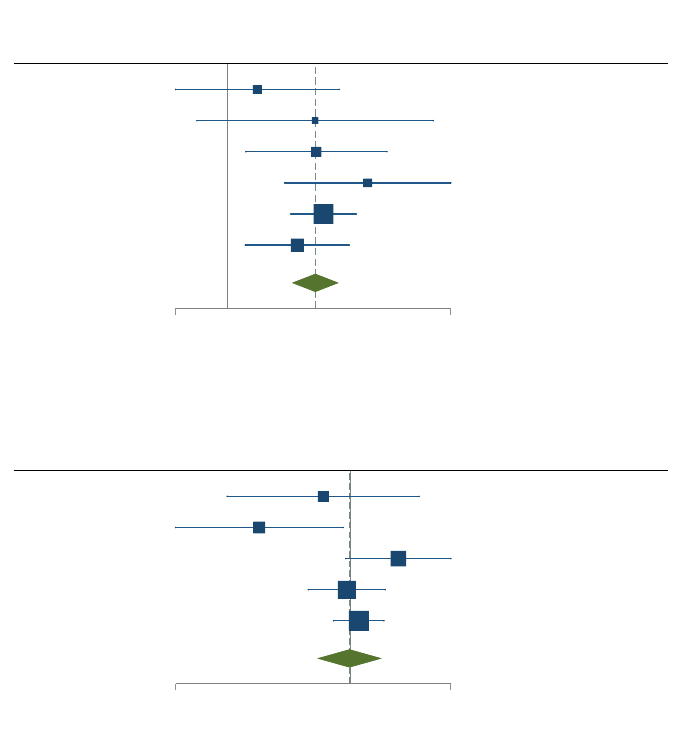
Figure 4: Effects on Recommended and Non-Recommended (Other) Inputs
KALRO
IPA/PxD1-Kenya
IPA/PxD2-Kenya
1AF1-Kenya
1AF2-Kenya
1AF3-Rwanda
Overall
Study
0.89 1.67
with 95% CI
Odds ratio
1.07 [
1.22 [
1.23 [
1.38 [
1.25 [
1.17 [
1.22 [
0.89,
0.93,
1.04,
1.14,
1.16,
1.04,
1.16,
1.29]
1.60]
1.44]
1.67]
1.34]
1.32]
1.29]
8.03
3.85
10.79
7.77
49.64
19.92
(%)
Weight
(a) Recommended Inputs
KALRO
IPA/PxD2-Kenya
1AF1-Kenya
1AF2-Kenya
1AF3-Rwanda
Overall
Study
0.66 1.27
with 95% CI
Odds ratio
0.94 [
0.81 [
1.12 [
0.99 [
1.02 [
1.00 [
0.75,
0.66,
0.99,
0.91,
0.96,
0.93,
1.18]
0.98]
1.27]
1.09]
1.08]
1.08]
8.87
10.93
19.92
26.47
33.81
(%)
Weight
(b) Non-Recommended (Other) Inputs
Notes: The figure plots the meta-analysis results for the effect of the programs on the use or purchases of recom-
mended inputs and other inputs not mentioned by the text-messages. The effects are estimated using a random-
effects meta-analysis model. Results are reported as odds ratios. The horizontal lines denote 95% confidence
intervals. Figure (a) reports results for recommended inputs. Figure (b) reports results for non-recommended
(other) inputs. IPA/PxD1-K is not included in (b) because no data for other non-recommended inputs was col-
lected in that case.
42

Figure 5: Effect Persistence Over Subsequent Season
KALRO
IPA/PxD2-Kenya
1AF1-Kenya
1AF3-Rwanda
Overall
Study
0.12
0.20
0.09
0.07
Control mean
0.53 1.72
with 95% CI
Odds ratio
0.87 [
1.23 [
1.02 [
1.06 [
1.06 [
0.53,
0.87,
0.68,
0.94,
0.95,
1.42]
1.72]
1.51]
1.20]
1.18]
4.67
9.88
7.29
78.16
(%)
Weight
(a) Lime: followed recommendations in second season
KALRO
IPA/PxD1-Kenya
IPA/PxD2-Kenya
1AF2-Kenya
Overall
Study
0.41
0.18
0.11
0.13
Control mean
0.73 1.74
with 95% CI
Odds ratio
1.12 [
1.28 [
0.96 [
1.07 [
1.08 [
0.83,
0.94,
0.73,
0.96,
0.99,
1.52]
1.74]
1.28]
1.20]
1.19]
9.20
8.99
10.68
71.13
(%)
Weight
(b) Fertilizer: followed recommendations in second season
Notes: The figure plots the meta-analysis results following lime and fertilizer recommendations in the second
season (for the subsamples that were only treated in the first season). The effects are estimated using a random-
effects meta-analysis model. Results are reported as odds ratios. The horizontal lines denote 95% confidence
intervals. Panel (a) reports results for following lime recommendations in the second season. Panel (b) reports
results for following fertilizer recommendations in the second season.
43

Figure 6: Message Fatigue
IPA/PxD1-Kenya
1AF1-Kenya
1AF3-Rwanda
Overall
Study
0.07
0.09
0.07
Control mean
0.69 1.87
with 95% CI
Odds ratio
1.12 [
1.27 [
1.30 [
1.29 [
0.69,
0.86,
1.15,
1.15,
1.80]
1.87]
1.48]
1.45]
5.86
8.83
85.31
(%)
Weight
(a) Lime: followed recommendations in second season
Notes: The figure plots the meta-analysis results following lime recommendations in the second season for the
subsample of farmers treated both in two subsequent seasons, compared to the control group. The effects are
estimated using a random-effects meta-analysis model. Results are reported as odds ratios. The horizontal lines
denote 95% confidence intervals.
44

Table 3: Summary of Meta-analytic Results
Effects Heterogeneity 95% Pred. Interval
# Outcome N Effect 95% CI Q stat (p) I
2
I
2
- 95% CI τ
2
(1) (2) (3) (4) (5) (6) (7) (8) (9) (10) (11)
Panel A. Effects from Logit specifications (odds ratios)
1 Awareness (Lime) 4 1.21 0.95 1.53 0.03 67.69 5.98 88.90 0.04 0.44 3.29
2 Knowledge (Acidity) 4 1.53 1.38 1.70 0.68 0.00 0.00 84.69 0.00 1.21 1.93
3 Lime Rec. 6 1.19 1.11 1.27 0.29 18.62 0.00 63.39 0.00 1.04 1.36
4 Fertilizer Rec. 4 1.27 1.15 1.40 0.67 0.00 0.00 84.69 0.00 1.03 1.57
5 Recommended Inputs 6 1.22 1.16 1.29 0.53 0.00 0.00 74.62 0.00 1.14 1.32
6 Other Inputs 5 1.00 0.93 1.08 0.08 51.89 0.00 82.32 0.00 0.80 1.25
7 Persistence Lime 4 1.06 0.95 1.18 0.71 0.00 0.00 84.69 0.00 0.84 1.34
8 Fatigue Lime 3 1.29 1.15 1.45 0.82 0.00 0.00 89.60 0.00 0.61 2.72
9 Persistence Fert. 4 1.08 0.99 1.19 0.60 0.00 0.00 84.69 0.00 0.88 1.33
Panel B. Effects from Linear Probability Models (percentage points)
10 Awareness (Lime) 4 0.03 -0.00 0.06 0.11 50.63 0.00 83.68 0.00 -0.09 0.14
11 Knowledge (Acidity) 4 0.08 0.04 0.12 0.04 64.31 0.00 87.92 0.00 -0.08 0.24
12 Lime Rec. 6 0.02 0.01 0.03 0.00 77.81 50.88 89.98 0.00 -0.02 0.06
13 Fert Rec. 4 0.01 0.00 0.03 0.02 70.00 13.82 89.56 0.00 -0.04 0.07
14 Recommended Inputs 6 0.02 0.01 0.03 0.00 81.20 59.68 91.23 0.00 -0.02 0.05
15 Other Inputs 5 0.00 -0.00 0.01 0.16 39.57 0.00 77.64 0.00 -0.01 0.01
16 Peristence Lime 4 0.00 -0.00 0.01 0.79 0.00 0.00 84.69 0.00 -0.01 0.02
17 Fatigue Lime 3 0.02 0.01 0.02 0.46 0.00 0.00 89.60 0.00 -0.03 0.07
18 Peristence Fert. 4 0.01 -0.00 0.02 0.50 0.00 0.00 84.69 0.00 -0.01 0.03
Panel C. Effects on quantity (Kg)
19 Kg Lime 6 1.18 0.10 2.27 0.00 86.15 71.97 93.15 1.29 -2.33 4.70
20 Kg Fertilizer 4 0.43 -0.03 0.89 0.02 70.31 14.85 89.64 0.12 -1.37 2.24
Notes: Meta-analysis results for each outcome reported in the rows. Column (1) reports the number of experiments included
in the meta-analyses. Columns (2)-(4) report results from a random-effects model. Columns (5)-(9) report heterogeneity re-
sults, and Columns (10)-(11) report prediction intervals. The coefficient represents the estimated summarized effects across
studies. Rows (1)-(9) report results measured in odds ratios. Rows (10)-(18) report results using linear probability models.
Rows (19)-(20) report results measured in kgs.
45
References
1AF (2014). Managing soil acidity with lime (2014 phase 2 trial report). Technical report, One
Acre Fund.
1AF (2015). Managing soil acidity with lime (2015 trial report). Technical report, One Acre
Fund.
1AF (2017). One acre fund: Annual report. Technical report, One Acre Fund.
1AF (2019). Lime experience trial results. One Acre Fund Report.
Aker, J. C. (2017). Using digital technology for public service provision in developing coun-
tries. Digital Revolutions in Public Finance, 201–24.
Aker, J. C., P. Collier, and P. C. Vicente (2017). Is information power? using mobile phones and
free newspapers during an election in Mozambique. Review of Economics and Statistics 99(2),
185–200.
Aker, J. C. and M. Fafchamps (2015). Mobile phone coverage and producer markets: Evidence
from West Africa. World Bank Economic Review 29(2), 262–292.
Aker, J. C., I. Ghosh, and J. Burrell (2016). The promise (and pitfalls) of ICT for agriculture
initiatives. Agricultural Economics 47(S1), 35–48.
Aker, J. C., C. Ksoll, and T. J. Lybbert (2012). Can mobile phones improve learning? evidence
from a field experiment in Niger. American Economic Journal: Applied Economics 4(4), 94–120.
Aker, J. C. and I. M. Mbiti (2010, September). Mobile phones and economic development in
Africa. Journal of Economic Perspectives 24(3), 207–32.
Allcott, H. (2015). Site selection bias in program evaluation. The Quarterly Journal of Eco-
nomics 130(3), 1117–1165.
Angrist, N., P. Bergman, and M. Matsheng (2020). School’s out: Experimental evidence on
limiting learning loss using “low-tech” in a pandemic. Technical report, National Bureau of
Economic Research.
46
Arouna, A., J. D. Michler, W. G. Yergo, and K. Saito (2019). One size does not fit all: Experi-
mental evidence on the digital delivery of personalized extension advice in nigeria.
Baum
¨
uller, H. (2018). The little we know: an exploratory literature review on the utility
of mobile phone-enabled services for smallholder farmers. Journal of International Develop-
ment 30(1), 134–154.
Beg, S., M. Islam, and K. W. Rahman (2024). Information and behavior: Evidence from fertil-
izer quantity recommendations in bangladesh. Journal of Development Economics 166, 103195.
Benartzi, S., J. Beshears, K. L. Milkman, C. R. Sunstein, R. H. Thaler, M. Shankar, W. Tucker-
Ray, W. J. Congdon, and S. Galing (2017). Should governments invest more in nudging?
Psychological science 28(8), 1041–1055.
BenYishay, A. and A. M. Mobarak (2019). Social learning and incentives for experimentation
and communication. The Review of Economic Studies 86(3), 976–1009.
Berazneva, J., L. McBride, M. Sheahan, and D. Guerena (2016). Perceived, measured, and
estimated soil fertility in east africa: Implications for farmers and researchers. Technical
report, Agricultural and Applied Economics Association.
Bettinger, E., N. Cunha, G. Lichand, and R. Madeira (2021). Are the effects of informational
interventions driven by salience? University of Zurich, Department of Economics, Working
Paper (350).
Bird, K. A., B. L. Castleman, J. T. Denning, J. Goodman, C. Lamberton, and K. O. Rosinger
(2019). Nudging at scale: Experimental evidence from fafsa completion campaigns. Journal
of Economic Behavior & Organization 183, 105–128.
Borenstein, M., L. Hedges, J. Higgins, and R. HR (2009). Introduction to Meta-Analysis. John
Wiley.
Borenstein, M., J. P. Higgins, L. V. Hedges, and H. R. Rothstein (2017). Basics of meta-analysis:
I2 is not an absolute measure of heterogeneity. Research synthesis methods 8(1), 5–18.
Brady, N. and R. Weil (2004). Soil acidity, alkalinity and salinity. Elements of the Nature and
Properties of Soils, 266–315.
47
Bujkiewicz, S., F. Achana, T. Papanikos, R. Riley, and K. Abrams (2019). Nice dsu technical
support document 20: multivariate meta-analysis of summary data for combining treatment
effects on correlated outcomes and evaluating surrogate endpoints. 2019. Availabe from:
https://www. sheffield.ac.uk/nice-dsu/tsds/full-list.
Buntaine, M. T., R. Jablonski, D. L. Nielson, and P. M. Pickering (2018). Sms texts on corruption
help ugandan voters hold elected councillors accountable at the polls. Proceedings of the
National Academy of Sciences 115(26), 6668–6673.
Bursztyn, L., S. Fiorin, D. Gottlieb, and M. Kanz (2019). Moral incentives in credit card debt
repayment: evidence from a field experiment. Journal of Political Economy 127(4), 1641–1683.
Camacho, A. and E. Conover (2010). The impact of receiving price and climate information in
the agricultural sector. Working Paper.
Casaburi, L., M. Kremer, S. Mullainathan, and R. Ramrattan (2014). Harnessing ICT to increase
agricultural production: Evidence from Kenya. Working Paper.
Chandrasekhar, A. G., E. Duflo, M. Kremer, J. F. Pugliese, J. Robinson, and F. Schilbach (2022).
Blue spoons: Sparking communication about appropriate technology use. Technical report,
National Bureau of Economic Research.
Chong, A., D. Karlan, J. Shapiro, and J. Zinman (2015). (ineffective) messages to encour-
age recycling: evidence from a randomized evaluation in peru. The World Bank Economic
Review 29(1), 180–206.
Chuang, E., P. Dupas, E. Huillery, and J. Seban (2020). Sex, lies, and measurement: Consistency
tests for indirect response survey methods. Journal of Development Economics 148, 102582.
Cole, S. A. and A. N. Fernando (2021). ‘mobile’izing agricultural advice technology adoption
diffusion and sustainability. The Economic Journal 131(633), 192–219.
Cooper, H., L. V. Hedges, and J. C. Valentine (2019). The handbook of research synthesis and
meta-analysis. Russell Sage Foundation.
Corral, C., X. Gin
´
e, A. Mahajan, and E. Seira (2020). Autonomy and specificity in agricultural
technology adoption: evidence from mexico. Technical report, National Bureau of Economic
Research.
48
Courtois, P. and J. Subervie (2014). Farmer bargaining power and market information services.
American Journal of Agricultural Economics 97(3), 953–977.
Cranados, G., S. Pandey, and H. Ceballos (1993). Response to selection for tolerance to acid
soils in a tropical maize population. Crop Science 33(5), 936–940.
Cunha, N., G. Lichand, R. Madeira, and E. Bettinger (2017). What is it about communicating
with parents? Working Paper.
Dahal, M. and N. Fiala (2020). What do we know about the impact of microfinance? the
problems of statistical power and precision. World Development 128, 104773.
Deeks, J. J. (2002). Issues in the selection of a summary statistic for meta-analysis of clinical
trials with binary outcomes. Statistics in medicine 21(11), 1575–1600.
Deichmann, U., A. Goyal, and D. Mishra (2016). Will digital technologies transform agriculture
in developing countries? Agricultural Economics 47(S1), 21–33.
DellaVigna, S. and E. Linos (2020). Rcts to scale: Comprehensive evidence from two nudge
units. Technical report, Working Paper, UC Berkeley.
DerSimonian, R. and N. Laird (1986). Meta-analysis in clinical trials. Controlled clinical tri-
als 7(3), 177–188.
Duflo, E., M. Kremer, and J. Robinson (2008). How high are rates of return to fertilizer?
evidence from field experiments in Kenya. The American Economic Review 98(2), 482–488.
Duflo, E., M. Kremer, and J. Robinson (2011). Nudging farmers to use fertilizer: Theory and
experimental evidence from kenya. The American Economic Review 101(6), 2350–2390.
Dustan, A., S. Maldonado, and J. M. Hernandez-Agramonte (2018). Motivating bureaucrats
with non-monetary incentives when state capacity is weak: Evidence from large-scale field
experiments in peru. Working Paper.
Emerick, K., A. de Janvry, E. Sadoulet, and M. H. Dar (2016). Identifying early adopters,
enhancing learning, and the diffusion of agricultural technology.
49

Engels, E. A., C. H. Schmid, N. Terrin, I. Olkin, and J. Lau (2000). Heterogeneity and sta-
tistical significance in meta-analysis: an empirical study of 125 meta-analyses. Statistics in
medicine 19(13), 1707–1728.
Fabregas, R; Kremer, M. R. J. S. F. (2019). The value of local agricultural information: The
value of local agricultural information: Evidence from kenya. Working paper.
Fabregas, R., M. Kremer, J. Robinson, and F. Schilbach (2017a). The effectiveness of public
agricultural extension: Evidence from two approaches in Kenya. Working Paper.
Fabregas, R., M. Kremer, J. Robinson, and F. Schilbach (2017b). Evaluating agricultural infor-
mation dissemination in western kenya (3ie impact evaluation report no. 67). New Delhi:
International Initiative for Impact Evaluation.
Fabregas, R., M. Kremer, and F. Schilbach (2019). Realizing the potential of digital develop-
ment: The case of agricultural advice. Science 366(6471).
Fafchamps, M. and B. Minten (2012). Impact of sms-based agricultural information on Indian
farmers. The World Bank Economic Review 26(3), 383–414.
FAO (2015). Status of the world’s soil resources (swsr)–main report. Food and agriculture
organization of the United Nations and intergovernmental technical panel on soils, Rome, Italy 650.
Friedman, W., B. Woodman, and M. Chatterji (2015). Can mobile phone messages to drug
sellers improve treatment of childhood diarrhoea?—a randomized controlled trial in ghana.
Health policy and planning 30(suppl 1), i82–i92.
Gelman, A., J. B. Carlin, H. S. Stern, D. B. Dunson, A. Vehtari, and D. B. Rubin (2013). Bayesian
data analysis. CRC press.
Gillwald, A. and O. Mothobi (2019). After access 2018: A demand-side view of mobile internet
from 10 african countries.
Glewwe, P., M. Kremer, S. Moulin, and E. Zitzewitz (2004). Retrospective vs. prospective anal-
yses of school inputs: the case of flip charts in kenya. Journal of development Economics 74(1),
251–268.
50
Grossman, G., M. Humphreys, and G. Sacramone-Lutz (2020). Information technology and
political engagement: Mixed evidence from uganda. The Journal of Politics 82(4), 1321–1336.
GSMA (2020). 10 years of mobile for development. Technical report.
Gudu, S., J. Okalebo, C. Othieno, P. Obura, D. Ligeyo, D. Shulze, and C. Johston (2005).
Response of five maize genotypes to nitrogen, phosphorus and lime on acid soils of Western
Kenya. In African Crop Science Conference Proceedings, Volume 7, pp. 1109–1115.
Gupta, A., J. Ponticelli, and A. Tesei (2020). Information, technology adoption and productiv-
ity: The role of mobile phones in agriculture. Technical report, National Bureau of Economic
Research.
Haaland, I., C. Roth, and J. Wohlfart (2020). Designing information provision experiments.
Hall, A. K., H. Cole-Lewis, and J. M. Bernhardt (2015). Mobile text messaging for health: a
systematic review of reviews. Annual Review of Public Health 36, 393–415.
Hall, B. H. and B. Khan (2003). Adoption of new technology.
Hall, C. S., E. Fottrell, S. Wilkinson, and P. Byass (2014). Assessing the impact of mhealth
interventions in low-and middle-income countries–what has been shown to work? Global
health action 7(1), 25606.
Hanna, R., S. Mullainathan, and J. Schwartzstein (2014). Learning through noticing: Theory
and evidence from a field experiment. The Quarterly Journal of Economics 129(3), 1311–1353.
Higgins, J. P., S. Green, et al. (2008). Cochrane handbook for systematic reviews of interven-
tions.
Higgins, J. P., J. Thomas, J. Chandler, M. Cumpston, T. Li, M. J. Page, and V. A. Welch (2019).
Cochrane handbook for systematic reviews of interventions. John Wiley & Sons.
Higgins, J. P. and S. G. Thompson (2002). Quantifying heterogeneity in a meta-analysis. Statis-
tics in medicine 21(11), 1539–1558.
Higgins, J. P., S. G. Thompson, J. J. Deeks, and D. G. Altman (2003). Measuring inconsistency
in meta-analyses. Bmj 327(7414), 557–560.
51
Hijbeek, R., M. P. van Loon, W. Ouaret, B. Boekelo, and M. K. van Ittersum (2021). Liming
agricultural soils in western kenya: Can long-term economic and environmental benefits
pay off short term investments? Agricultural Systems 190, 103095.
Ioannidis, J., T. Stanley, and H. Doucouliagos (2017). The power of bias in economics research.
The Economic Journal 127(605), F236–F265.
Jamison, J. C., D. Karlan, and P. Raffler (2013). Mixed-method evaluation of a passive mhealth
sexual information texting service in uganda. Information Technologies & International Devel-
opment 9(3), pp–1.
Jensen, R. (2007). The digital provide: Information (technology), market performance, and
welfare in the south Indian fisheries sector. The Quarterly Journal of Economics.
Kamprath, E. (1970). Exchangeable aluminum as a criterion for liming leached mineral soils.
Soil Science Society of America Journal 34(2), 252–254.
Kanyanjua, S., L. Ireri, S. Wambua, and S. Nandwa (2002). Acidic soils in kenya: Constraints
and remedial options. KARI Technical Note No. 11.
Kanyanjua, S. M., S. L. Ireri, Wambua, and S. Nandwa. (2002). Kari technical note no. 11,
acidic soils in Kenya: constraints and remedial options. KARI Headquarters, Nairobi, Kenya.
Karlan, D., M. McConnell, S. Mullainathan, and J. Zinman (2016). Getting to the top of mind:
How reminders increase saving. Management Science 62(12), 3393–3411.
Karlan, D., M. Morten, and J. Zinman (2012). A personal touch: Text messaging for loan
repayment. Technical report, National Bureau of Economic Research.
Karlan, D., M. Morten, and J. Zinman (2015). A personal touch in text messaging can improve
microloan repayment. Behavioral Science & Policy 1(2), 25–31.
Karlan, D. and J. Zinman (2008). Lying about borrowing. Journal of the European Economic
Association 6(2-3), 510–521.
Karlan, D. S. and J. Zinman (2012). List randomization for sensitive behavior: An application
for measuring use of loan proceeds. Journal of Development Economics 98(1), 71–75.
52
Kelly, V. and A. Murekezi (2000). Fertilizer response and profitability in rwanda. A Synthesis
of Findings from MINAGRI Studies Conducted by the Food Security Research Project (FSRP) and
the FAO Soil Fertility Initiative. Kigali, Rwanda: FSRP/MINAGRI, February.
Kisinyo, P., P. Opala, V. Palapala, S. Gudu, C. Othieno, and E. Ouma (2015). Micro-dosing
of lime, phosphorus and nitrogen fertilizers effect on maize performance on an acid soil in
Kenya. Sustainable Agriculture Research 4(2), 21.
Kling, J. R., J. B. Liebman, and L. F. Katz (2007). Experimental analysis of neighborhood effects.
Econometrica 75(1), 83–119.
KSHC (2014). Policy brief: Soil health research gaps in kenya.
https://www.kalro.org/sites/default/files/KSHC
Larochelle, C., J. Alwang, E. Travis, V. H. Barrera, and J. M. D. Andrade (2019). Did you really
get the message? Using text reminders to stimulate adoption of agricultural technologies.
The Journal of Development Studies 55(4), 548–564.
Lobell, D. B., G. Azzari, M. Burke, S. Gourlay, Z. Jin, T. Kilic, and S. Murray (2018). Eyes in the
sky, boots on the ground: assessing satellite-and ground-based approaches to crop yield measurement
and analysis in Uganda. The World Bank.
Marenya, P. P. and C. B. Barrett (2009). State-conditional fertilizer yield response on Western
Kenyan farms. American Journal of Agricultural Economics 91(4), 991–1006.
McKenzie, D. and C. Woodruff (2014). What are we learning from business training and
entrepreneurship evaluations around the developing world? The World Bank Research Ob-
server 29(1), 48–82.
Meager, R. (2019). Understanding the average impact of microcredit expansions: A bayesian
hierarchical analysis of seven randomized experiments. American Economic Journal: Applied
Economics 11(1), 57–91.
Mitra, S., D. Mookherjee, M. Torero, and S. Visaria (2017). Asymmetric information and
middleman margins: An experiment with Indian potato farmers. Review of Economics and
Statistics (0).
53
Muralidharan, K., M. Romero, and K. W
¨
uthrich (2020). Factorial designs, model selection,
and (incorrect) inference in randomized experiments. The Review of Economics and Statistics,
1–44.
NAAIAP (2014). Soil suitability evaluation for maize production in kenya.
https://africafertilizer.org/wp-content/uploads/2017/04/Soil-Suitability-Evaluation-
for-Maize-Prod.-in-Kenya.pdf.
Nakasone, E., M. Torero, and B. Minten (2014). The power of information: The ICT revolution
in agricultural development. Annu. Rev. Resour. Econ. 6(1), 533–550.
Nduwumuremyi, A., S. Habimana, T. Alexis, and J. Mupenzi (2014). Soil acidity analysis and
estimation of lime requirement for rectifying soil acidity. International Invention Journal of
Agricultural and Soil Science 2(2), 22–26.
Omenyo, V. S., J. Okalebo, and C. Othieno (2018). Effects of lime and phosphorus fertilizer on
maize performance in acid soils of western Kenya. Second RUFORUM Biennial Meeting 20 -
24 September 2010, Entebbe, Uganda.
Oreopoulos, P. and U. Petronijevic (2019). The remarkable unresponsiveness of college stu-
dents to nudging and what we can learn from it. Technical report, National Bureau of
Economic Research.
Pop-Eleches, C., H. Thirumurthy, J. P. Habyarimana, J. G. Zivin, M. P. Goldstein, D. De Walque,
L. Mackeen, J. Haberer, S. Kimaiyo, J. Sidle, et al. (2011). Mobile phone technologies improve
adherence to antiretroviral treatment in a resource-limited setting: a randomized controlled
trial of text message reminders. AIDS (London, England) 25(6), 825.
Pritchett, L. and J. Sandefur (2015). Learning from experiments when context matters. Ameri-
can Economic Review 105(5), 471–75.
Raifman, J. R., H. E. Lanthorn, S. Rokicki, and G. Fink (2014). The impact of text message
reminders on adherence to antimalarial treatment in northern ghana: a randomized trial.
PloS one 9(10), e109032.
Rokicki, S., J. Cohen, J. A. Salomon, and G. Fink (2017). Impact of a text-messaging program
54
on adolescent reproductive health: a cluster–randomized trial in ghana. American journal of
public health 107(2), 298–305.
Rosenzweig, M. R. and C. Udry (2020). External validity in a stochastic world: Evidence from
low-income countries. The Review of Economic Studies 87(1), 343–381.
Rubin, D. (1981). Estimation in parallel randomized experiments. Journal of Educational and
Behavioral Statistics.
Schmidt, S. and M. Eisend (2015). Advertising repetition: A meta-analysis on effective fre-
quency in advertising. Journal of Advertising 44(4), 415–428.
Sheahan, M. and C. B. Barrett (2017). Ten striking facts about agricultural input use in sub-
saharan africa. Food Policy 67, 12–25.
Steinhardt, L. C., D. P. Mathanga, D. Mwandama, H. Nsona, D. Moyo, A. Gumbo,
M. Kobayashi, R. Namuyinga, M. P. Shah, A. Bauleni, et al. (2019). The effect of text mes-
sage reminders to health workers on quality of care for malaria, pneumonia, and diarrhea
in malawi: a cluster-randomized, controlled trial. The American journal of tropical medicine
and hygiene 100(2), 460–469.
Suri, T. (2011). Selection and comparative advantage in technology adoption. Economet-
rica 79(1), 159–209.
Svensson, J. and D. Yanagizawa (2009). Getting prices right: the impact of the market infor-
mation service in uganda. Journal of the European Economic Association 7(2-3), 435–445.
The, C., H. Calba, E. L. M. Zonkeng, C.and Ngonkeu, and V. O. Adetimirin (2006). Response
of maize grain yield to changes in acid soil characteristics after soil amendment. Plant Soil.
Tisdale, S. L., W. L. Nelson, and J. D. Beaton (1990). Soil fertility and fertilizers. New York:
Macmillan.
Tjernstr
¨
om, E., T. J. Lybbert, R. F. Hern
´
andez, and J. S. Correa (2019). Learning by (virtually)
doing: experimentation and belief updating in smallholder agriculture. Technical report,
Working Paper, University of Wisconsin-Madison.
UNESCO (2022). Institute for statistics (uis) database.
55
Van Campenhout, B., D. J. Spielman, and E. Lecoutere (2020). Information and communication
technologies to provide agricultural advice to smallholder farmers: Experimental evidence
from uganda. American Journal of Agricultural Economics.
Vivalt, E. (2016). How much can we generalize from impact evaluations? Working Paper.
Wiecek, W. and R. Meager (2022). baggr: Bayesian aggregation package for r, v0.6.16.
https://github.com/wwiecek/baggr.
56

Online Appendix
Table of Contents
A Projects Map 58
B Regression Controls and Variables 59
C Attrition & Balance 60
D Results by Experiment: Pooled Treatment Arms 67
E Pooled Regressions 75
F Results by Experiment: By Treatment Arms 77
G Cost-Benefit and Cost-Effectiveness 80
G.1 Cost-effectiveness . . . . . . . . . . . . . . . . . . . . . . . . . . . . . . . . . . . . 80
G.2 Cost-benefit . . . . . . . . . . . . . . . . . . . . . . . . . . . . . . . . . . . . . . . 81
H Heterogeneity by Experiment 84
I Additional Meta-analyses 86
I.1 Bayesian Meta-analysis . . . . . . . . . . . . . . . . . . . . . . . . . . . . . . . . 90
J Additional Program and Experiment Details 93
J.1 KALRO’s Program . . . . . . . . . . . . . . . . . . . . . . . . . . . . . . . . . . . 93
J.2 IPA & PxD’s Programs . . . . . . . . . . . . . . . . . . . . . . . . . . . . . . . . . 95
J.3 One Acre Fund’s Programs . . . . . . . . . . . . . . . . . . . . . . . . . . . . . . 99
K Agricultural Recommendations 104
K.1 Generating Agricultural Recommendations . . . . . . . . . . . . . . . . . . . . . 104
K.2 Considerations in Using Area-level Information to Generate Agricultural Advice107
57

A Projects Map
Figure A1: Projects Map
(a) western Kenya
(b) Rwanda
Notes: Panel (a) shows the median level of pH in all wards (geographical areas) and the location of the programs
in Kenya. Panel (b) shows the sectors in Rwanda in which the 1AF3-R program took place and the median level
of pH, where available.
58

B Regression Controls and Variables
Table B1: Data Collected on Inputs, Control Variables and Strata
Sample Recommended Inputs Non-Recommended Inputs Control Variables
Other Fertilizers Strata Other
KALRO
lime, planting fertilizer
(DAP, NPK), top-dressing
fertilizer (CAN, Mavuno),
compost, manure, hybrid
seeds, weed
control, intercropping
test acidity
grain storage
rhizobia
pest and
disease control,
improved legumes
female, lime awareness,
input use index (tercile),
grew legumes,
farm size (median)
cognitive score (tercile),
school area FE
prior soil testing,
enumerator FE
IPA/PxD1-K lime, DAP, urea
NPK,
CAN,
Mavuno
female, database origin,
farm size (tercile)
ag. knowledge
(median), prior
urea use,
prior lime use,
positive valuation
completed poll,
area FE
age,
primary education
language,
safaricom
phone network,
enumerator FE
(survey outcomes)
IPA/PxD2-K
lime, DAP, urea
(mentioned CAN use
for poor rains)
hybrid seeds,
pesticides
NPK,
Mavuno
female,
prior lime use,
agrovet recruiter FE
age, land size,
language,
farmer area FE,
enumerator FE
(survey outcomes)
1AF1-K lime
actellic, compost,
drying sheets,
storage bags
extra CAN
maize package
(acres),
seasons in
1AF, group size,
prior purchase of
extra CAN,
area FE,
enumerator FE
(survey outcomes)
1AF2-K lime, extra CAN
actellic, compost,
drying sheets,
storage bags
seasons in 1AF,
area FE
maize package
(acres),
seasons in
1AF, group size,
prior purchase of
extra CAN,
prior lime purchase,
area FE
1AF3-R lime
DAP, NPK, urea,
storage bags
seasons in 1AF,
group size,
prior lime purchase,
area FE
Notes: The table shows the list of recommended inputs for each program for which we have administrative or survey data at endline, the
list of non-recommended (not mentioned) inputs for which we have survey data at endline, and the list of randomization strata included in
the main specifications when estimating impacts for each program, as well as the list of additional control variables included in the robust-
ness specifications (all of them measured prior to the program introduction). Included controls are constrained by data availability for each
project. FE denotes fixed effects.
59

C Attrition & Balance
Table C1: KALRO: Summary Statistics & Balance
Control Treated (1) vs. (2)
(1) (2) (3)
Age 41.85 40.41 1.44
(0.67) (0.67) (0.95)
Female 0.65 0.66 -0.01
(0.02) (0.02) (0.03)
Primary school 0.51 0.54 -0.03
(0.03) (0.03) (0.04)
Secondary school 0.03 0.04 -0.01
(0.01) (0.01) (0.01)
Footwear 0.60 0.56 0.04
(0.03) (0.03) (0.04)
Mumias 0.57 0.57 -0.01
(0.03) (0.03) (0.04)
Acres (owned and rented) 2.25 1.98 0.27
(0.28) (0.10) (0.30)
Literate 0.90 0.91 0.00
(0.02) (0.01) (0.02)
Had soil test 0.13 0.11 0.02
(0.02) (0.02) (0.02)
Mentions lime 0.03 0.04 -0.01
(0.01) (0.01) (0.01)
Used lime 0.07 0.07 0.00
(0.01) (0.01) (0.02)
Used fertilizer last LR season 0.84 0.84 0.00
(0.02) (0.02) (0.03)
Grew legumes last LR season 0.79 0.77 0.02
(0.02) (0.02) (0.03)
Heard lime 0.40 0.41 0.00
(0.03) (0.02) (0.04)
Heard soil test 0.67 0.72 -0.05
(0.02) (0.02) (0.03)
Ever used DAP 0.94 0.94 0.00
(0.01) (0.01) (0.02)
Ever used CAN 0.61 0.64 -0.03
(0.02) (0.02) (0.03)
Ever used NPK 0.12 0.15 -0.03
(0.02) (0.02) (0.02)
N 384 389 773
Joint F-Stat (w/strata) 1.119
p-value 0.33
Joint F-Stat (w/controls & FE) 1.206
p-value 0.27
Notes: The table shows summary statistics by treatment group and their differences using
data from the baseline survey. The sample is restricted to non-attriting observations from
the endline survey. Columns (1)–(2) display the mean and standard error of each character-
istic for each treatment group. Column (3) displays the differences across columns and the
corresponding standard error. Primary school and Secondary school refer to completing pri-
mary and secondary education, respectively. Footwear denotes whether the respondent was
wearing shoes (a proxy for income) at the time of the survey. Mumias denotes the share of
farmers from the Mumias area, Had soil test denotes ever having a soil test, Mentions Lime is
a dummy variable with value one if the respondent mentioned lime as a strategy to reduce
soil acidity. Heard soil test and Heard Lime take the value one if the respondent has ever heard
of using soil tests to test for acidity or has heard about lime, respectively. The joint F-stat
(w/strata) and p-value refer to a test of the joint significance of baseline variables, exclud-
ing those used as strata (see Table B1) using a specification that matches that of the main
analysis, including strata. The joint F-stat (w/add.controls & FE) refers to a test of the joint
significance of baseline variables excluding those used as controls, using a specification that
includes controls, strata, area, and enumerator fixed effects.
∗
p < .10,
∗∗
p < .05,
∗∗∗
p < .01.
60

Table C2: IPA/PxD1-K: Summary Statistics & Balance
Control General Specific (1) vs. (2) (1) vs. (3) (2) vs. (3)
(1) (2) (3) (4) (5) (6)
Age 46.25 46.01 45.59 0.25 0.66 0.42
(0.49) (0.45) (0.43) (0.66) (0.65) (0.63)
Female 0.37 0.37 0.37 -0.01 0.00 0.00
(0.02) (0.02) (0.02) (0.03) (0.03) (0.03)
Primary school 0.60 0.61 0.66 -0.01 -0.05* -0.04
(0.02) (0.02) (0.02) (0.03) (0.03) (0.03)
Secondary school 0.10 0.10 0.10 0.00 0.01 0.01
(0.01) (0.01) (0.01) (0.02) (0.02) (0.02)
Mumias 0.53 0.53 0.53 0.00 0.00 0.00
(0.02) (0.02) (0.02) (0.03) (0.03) (0.03)
Prefers english 0.30 0.27 0.30 0.03 0.00 -0.03
(0.02) (0.02) (0.02) (0.03) (0.03) (0.03)
Mentions lime 0.16 0.17 0.17 0.00 0.00 0.00
(0.01) (0.01) (0.01) (0.02) (0.02) (0.02)
Acres (owned and rented) 2.00 1.86 2.14 0.14 -0.14 -0.28
(0.09) (0.08) (0.31) (0.12) (0.32) (0.32)
Used lime 0.12 0.13 0.12 -0.01 0.00 0.01
(0.01) (0.01) (0.01) (0.02) (0.02) (0.02)
Used DAP last LR season 0.78 0.78 0.80 0.00 -0.02 -0.02
(0.02) (0.02) (0.02) (0.02) (0.02) (0.02)
Used NPK last LR season 0.04 0.05 0.04 -0.01 0.00 0.01
(0.01) (0.01) (0.01) (0.01) (0.01) (0.01)
Used CAN last LR season 0.62 0.62 0.59 0.00 0.02 0.02
(0.02) (0.02) (0.02) (0.03) (0.03) (0.03)
Used urea last LR season 0.18 0.18 0.18 0.00 0.00 0.00
(0.02) (0.02) (0.02) (0.02) (0.02) (0.02)
Used mavuno last LR season 0.15 0.13 0.16 0.02 -0.01 -0.03
(0.01) (0.01) (0.01) (0.02) (0.02) (0.02)
Enrolled in main phone network 0.95 0.94 0.94 0.01 0.01 0.00
(0.01) (0.01) (0.01) (0.01) (0.01) (0.01)
Lime recommended 0.82 0.82 0.82 0.00 0.00 0.00
(0.02) (0.02) (0.02) (0.02) (0.02) (0.02)
N 632 633 632 1265 1264 1265
Joint F-Stat (w/ strata) 0.504 1.044 1.229
p-value 0.913 0.405 0.257
Joint F-Stat (w/add. controls & FE) 0.332 0.892 1.542
p-value 0.954 0.522 0.138
Notes: The table shows summary statistics and balance tests using covariate variables from a baseline survey. Columns (1)–(3)
display the mean and standard error of each characteristic for each treatment group. Columns (4)-(6) display the difference
across columns and the corresponding standard error. Mumias denotes the share of farmers from the Mumias Sugar Com-
pany sample. pH prediction represents the median pH level measured in the farmer’s catchment area. Mentions Lime is a
dummy variable with value one if the respondent mentioned lime as a strategy to reduce soil acidity. Input use variables
refer to whether respondents used the specific input during the previous long rain (LR) season. Lime recommended indicates
whether the farmer resided in an area where the use of lime was recommended. The joint F-stat (w/strata) and p-value refer
to a test of the joint significance of baseline variables, excluding those used as randomization strata (see Table B1) using a
specification that matches that of the main analysis, including strata. The joint F-stat (w/add.controls & FE) refers to a test of
the joint significance of baseline variables excluding those used as controls, using a specification that includes controls, strata,
and area-fixed effects.
∗
p < .10,
∗∗
p < .05,
∗∗∗
p < .01.
61

Table C3: IPA/PxD2-K: Additional Summary Statistics & Balance
Control SMS SMS+Call SMS+Call Offer (1) vs. (2) (1) vs. (3) (1) vs. (4)
(1) (2) (3) (4) (5) (6) (7)
Age 42.10 41.40 41.48 41.44 0.70 0.61 0.66
(0.32) (0.31) (0.32) (0.31) (0.45) (0.46) (0.45)
Female 0.34 0.34 0.34 0.34 0.00 0.00 0.00
(0.01) (0.01) (0.01) (0.01) (0.02) (0.02) (0.02)
Primary school 0.72 0.70 0.69 0.71 0.01 0.02 0.01
(0.01) (0.01) (0.01) (0.01) (0.02) (0.02) (0.02)
Secondary school 0.13 0.13 0.12 0.13 -0.01 0.01 0.00
(0.01) (0.01) (0.01) (0.01) (0.01) (0.01) (0.01)
Prefers english 0.36 0.35 0.34 0.35 0.01 0.02 0.01
(0.01) (0.01) (0.01) (0.01) (0.02) (0.02) (0.02)
Mentions lime 0.26 0.26 0.24 0.25 0.00 0.01 0.01
(0.01) (0.01) (0.01) (0.01) (0.02) (0.02) (0.02)
Acres (owned and rented) 2.02 1.85 2.09 2.03 0.17** -0.07 -0.02
(0.06) (0.05) (0.09) (0.06) (0.08) (0.11) (0.08)
Used lime 0.09 0.09 0.09 0.10 -0.01 0.00 -0.01
(0.01) (0.01) (0.01) (0.01) (0.01) (0.01) (0.01)
Used CAN last LR season 0.64 0.62 0.65 0.62 0.02 0.00 0.02
(0.01) (0.01) (0.01) (0.01) (0.02) (0.02) (0.02)
Used urea last LR season 0.18 0.20 0.20 0.18 -0.02 -0.02 0.00
(0.01) (0.01) (0.01) (0.01) (0.01) (0.01) (0.01)
Used mavuno last LR season 0.08 0.08 0.07 0.09 0.00 0.01 0.00
(0.01) (0.01) (0.01) (0.01) (0.01) (0.01) (0.01)
Lime recommended 0.77 0.76 0.77 0.76 0.01 0.00 0.01
(0.01) (0.01) (0.01) (0.01) (0.02) (0.02) (0.02)
N 1470 1475 1473 1472 2945 2943 2942
Joint F-Stat (w/strata) 0.991 1.183 0.681
p-value 0.449 0.297 0.743
Joint F-Stat (w/add. controls & FE) 0.632 0.872 0.391
p-value 0.705 0.514 0.885
Notes: The table shows summary statistics and balance tests using covariate variables from a baseline survey. Columns (1)–(4) display the
mean and standard error of each characteristic for each treatment group. Columns (5)-(7) display the difference across columns and the corre-
sponding standard error. pH prediction represents the median pH level measured in the farmer’s ward used to provide lime recommendations.
Prefers english indicates respondent preferred messages in English rather than Swahili. Mentions Lime is a dummy variable with value one if
the respondent mentioned lime as a strategy to reduce soil acidity. Input use variables refer to whether respondents used the specific input
during the previous long rain (LR) season. Lime recommended indicates whether the farmer resided in an area where the use of lime was rec-
ommended. The joint F-stat (w/strata) and p-value refer to a test of the joint significance of baseline variables, excluding those used as strata
(see Table B1) using a specification that matches that of the main analysis, including strata. The joint F-stat (w/add.controls & FE) refers to a
test of the joint significance of baseline variables excluding those used as controls, using a specification that includes controls, strata, area, and
agrovet-fixed effects.
∗
p < .10,
∗∗
p < .05,
∗∗∗
p < .01.
62

Table C4: 1AF1-K: Additional Summary Statistics & Balance
Broad Control Detailed (1) vs. (2) (1) vs. (3) (2) vs. (3)
(1) (2) (3) (4) (5) (6)
Female 0.64 0.64 0.67 0.00 -0.02 -0.03
(0.01) (0.01) (0.01) (0.02) (0.02) (0.02)
Group size 9.24 9.08 9.07 0.16 0.17* 0.01
(0.07) (0.07) (0.07) (0.10) (0.10) (0.10)
1AF seasons 1.50 1.51 1.52 0.00 -0.02 -0.02
(0.02) (0.02) (0.02) (0.03) (0.03) (0.03)
Maize inputs (acres) 0.49 0.50 0.50 -0.01 -0.02 -0.01
(0.01) (0.01) (0.01) (0.01) (0.01) (0.01)
pH prediction 5.48 5.48 5.48 0.00 0.01 0.01
(0.01) (0.01) (0.01) (0.01) (0.01) (0.01)
Intercropped beans 0.03 0.03 0.03 0.01 0.01 0.00
(0.00) (0.00) (0.00) (0.01) (0.01) (0.01)
Extra CAN purchased 0.10 0.08 0.10 0.02* 0.00 -0.02*
(0.01) (0.01) (0.01) (0.01) (0.01) (0.01)
Repayment incentive 0.05 0.04 0.04 0.01 0.01 0.00
(0.01) (0.01) (0.00) (0.01) (0.01) (0.01)
Storage bags 0.09 0.07 0.07 0.02** 0.02** 0.00
(0.01) (0.01) (0.01) (0.01) (0.01) (0.01)
PICS bags 0.08 0.08 0.09 0.00 -0.01 -0.01
(0.01) (0.01) (0.01) (0.01) (0.01) (0.01)
Compost booster 0.05 0.05 0.05 0.00 0.00 0.00
(0.01) (0.01) (0.01) (0.01) (0.01) (0.01)
Red onions 0.11 0.07 0.10 0.03*** 0.01 -0.02**
(0.01) (0.01) (0.01) (0.01) (0.01) (0.01)
Reusable pads 0.05 0.04 0.04 0.01 0.00 0.00
(0.01) (0.00) (0.00) (0.01) (0.01) (0.01)
Drying sheets 0.24 0.23 0.24 0.01 0.00 -0.01
(0.01) (0.01) (0.01) (0.01) (0.01) (0.01)
Actellic super 0.10 0.09 0.11 0.01 -0.01 -0.02
(0.01) (0.01) (0.01) (0.01) (0.01) (0.01)
Solar lamps 0.46 0.45 0.46 0.01 -0.01 -0.01
(0.01) (0.01) (0.01) (0.02) (0.02) (0.02)
Health insurance 0.23 0.22 0.21 0.01 0.02 0.01
(0.01) (0.01) (0.01) (0.01) (0.01) (0.01)
N 1684 1559 1641 3243 3325 3200
Joint F-Stat (w/strata) 1.448 0.978 1.428
p-value 0.104 0.480 0.113
Joint F-Stat (w/add. controls & FE) 1.466 0.940 1.512
p-value 0.122 0.510 0.105
Notes: The table shows summary statistics and balance tests using covariate variables from 1AF long rain 2016 administra-
tive records (before the trial took place). Columns (1)-(3) display mean and standard errors of each variable, by treatment
group. Columns (4)-(6) display the difference across columns and the corresponding standard error. Group size denotes the
number of farmers in the participant’s 1AF group, 1AF seasons denotes the number of denotes the number of prior seasons of
enrollment in the 1AF program, in the 1AF program, Maize inputs (acres) refers to the size, in acres, of the agricultural inputs
package purchased from 1AF, pH prediction is the variable obtained using kriging interpolation that was used to produce de-
tailed recommendations, Intercropped beans,Extra CAN purchased, Repayment incentive, Storage bags, PICS bags, Compost booster,
Red onions, Drying sheets, Reusable pads,Actellic super, Solar lamps and Health insurance are dummy variables equal to one if
the farmer had purchased or received any of those products from 1AF in the season prior to the experiment. Differences in
variables across 1AF balance tables stems from differences in shared variables by project and/or differences in regional pro-
grams. The joint F-stat (w/strata) and p-value refer to a test of the joint significance of baseline variables, excluding those
used as strata if strata were used in the randomization (see Table B1) using a specification that matches that of the main
analysis. The joint F-stat (w/add.controls & FE) refers to a test of the joint significance of baseline variables excluding those
used as controls, using a specification that includes controls and area-fixed effects.
∗
p < .10,
∗∗
p < .05,
∗∗∗
p < .01.

Table C5: 1AF2-K: Summary Statistics & Balance
Control Lime + CAN Lime only (1) vs. (2) (1) vs. (3) (2) vs. (3)
(1) (2) (3) (4) (5) (6)
Age 48.40 48.44 48.30 -0.04 0.10 0.14
(0.15) (0.20) (0.10) (0.25) (0.18) (0.22)
Female 0.69 0.68 0.69 0.01 0.00 -0.01
(0.01) (0.01) (0.00) (0.01) (0.01) (0.01)
Group size 9.87 9.92 9.82 -0.05 0.04 0.10**
(0.03) (0.04) (0.02) (0.05) (0.04) (0.05)
1AF seasons 2.23 2.22 2.23 0.01 0.00 -0.01
(0.02) (0.02) (0.01) (0.03) (0.02) (0.02)
Maize inputs (acres) 0.51 0.53 0.51 -0.01** 0.00 0.01**
(0.00) (0.00) (0.00) (0.01) (0.00) (0.01)
pH prediction 5.33 5.33 5.33 0.00 0.00 0.00
(0.00) (0.00) (0.00) (0.00) (0.00) (0.00)
Intercropped beans 0.02 0.02 0.02 0.00 0.00 0.00
(0.00) (0.00) (0.00) (0.00) (0.00) (0.00)
Extra CAN purchased 0.15 0.14 0.15 0.01 0.00 -0.01
(0.00) (0.01) (0.00) (0.01) (0.00) (0.01)
Repayment incentive 0.04 0.05 0.05 0.00 -0.01*** -0.01**
(0.00) (0.00) (0.00) (0.00) (0.00) (0.00)
Storage bags 0.11 0.11 0.12 0.00 0.00 -0.01
(0.00) (0.00) (0.00) (0.01) (0.00) (0.01)
PICS bags 0.09 0.09 0.09 0.00 0.00 0.00
(0.00) (0.00) (0.00) (0.01) (0.00) (0.00)
Compost booster 0.04 0.04 0.04 0.00 0.00 0.00
(0.00) (0.00) (0.00) (0.00) (0.00) (0.00)
Red onions 0.03 0.04 0.03 0.00 0.00 0.00
(0.00) (0.00) (0.00) (0.00) (0.00) (0.00)
Reusable pads 0.03 0.03 0.03 0.00 0.00 0.00
(0.00) (0.00) (0.00) (0.00) (0.00) (0.00)
Drying sheets 0.22 0.23 0.22 -0.01 0.00 0.01
(0.00) (0.01) (0.00) (0.01) (0.01) (0.01)
Actellic 0.18 0.18 0.18 0.00 0.00 0.00
(0.00) (0.01) (0.00) (0.01) (0.01) (0.01)
Solar lamps 0.42 0.43 0.42 0.00 0.00 0.01
(0.01) (0.01) (0.00) (0.01) (0.01) (0.01)
Credit size (Ksh) 9501.74 9616.95 9466.33 -115.21 35.41 150.62**
(49.86) (64.63) (31.67) (81.57) (58.69) (71.19)
N 8142 4872 19558 13014 27700 24430
Joint F-Stat (w/ strata) 1.190 0.964 1.844
p-value 0.267 0.494 0.021
Joint F-Stat (w/add. controls & FE) 1.284 0.580 1.308
p-value 0.214 0.872 0.199
Notes: The table shows summary statistics and balance tests using covariate variables from 1AF long rain 2017 administrative records
(before the trial took place). Columns (1)-(3) display mean and standard errors of each variable, by treatment group. Columns (4)-(6)
display the difference across columns and the corresponding standard error. Group size denotes the number of farmers in the partici-
pant’s 1AF group, 1AF seasons denotes the number of denotes the number of prior seasons of enrollment in the 1AF program, in the
1AF program, Maize inputs (acres) refers to the size, in acres, of the agricultural inputs package purchased from 1AF, pH prediction is
the variable obtained using kriging interpolation that was used to produce detailed recommendations, Intercropped beans,Extra CAN
purchased, Repayment incentive, Storage bags, PICS bags, Compost booster, Red onions, Drying sheets, Reusable pads,Actellic super and Solar
lamps are dummy variables equal to one if the farmer had purchased or received any of those products from 1AF in the season prior
to the experiment. Credit size is the size of credit in Kenyan shillings taken from 1AF in the season prior to the experiment. The joint
F-stat (w/strata) and p-value refer to a test of the joint significance of baseline variables, excluding those used as strata (see Table B1)
using a specification that matches that of the main analysis, including strata. The joint F-stat (w/add.controls & FE) refers to a test
of the joint significance of baseline variables excluding those used as controls, using a specification that includes controls, strata and
area-fixed effects.
∗
p < .10,
∗∗
p < .05,
∗∗∗
p < .01.

65
Table C6: 1AF3-R: Summary Statistics & Balance
Full Control Full Treatment Partial Treatment (1) vs. (2) (1) vs. (3) (1) vs. (4)
Non Treated Treated
(1) (2) (3) (4) (5) (6) (7)
Group size 10.71 10.75 10.72 10.71 -0.04 -0.01 -0.00
(0.06) (0.05) (0.04) (0.04) (0.08) (0.08) (0.07)
1AF seasons 2.01 2.01 2.01 2.01 -0.00 -0.00 0.00
(0.02) (0.02) (0.02) (0.02) (0.03) (0.03) (0.03)
Purchased lime 0.06 0.06 0.06 0.06 0.00 0.01
∗
0.01
∗
(0.00) (0.00) (0.00) (0.00) (0.00) (0.00) (0.00)
Purchased urea 0.74 0.74 0.74 0.74 -0.00 0.01 -0.00
(0.01) (0.00) (0.00) (0.00) (0.01) (0.01) (0.01)
Planting fertilizer (kg) 13.71 13.80 13.64 13.71 -0.09 0.07 -0.00
(0.20) (0.14) (0.14) (0.14) (0.25) (0.24) (0.24)
Seeds (kg) 2.49 2.43 2.45 2.45 0.06 0.04 0.04
(0.04) (0.03) (0.03) (0.03) (0.05) (0.05) (0.05)
PICS bags 0.06 0.07 0.07 0.07 -0.00 -0.00 -0.00
(0.00) (0.00) (0.00) (0.00) (0.00) (0.00) (0.00)
Solar Lamp 0.28 0.27 0.29 0.28 0.01 -0.01 -0.00
(0.01) (0.00) (0.00) (0.00) (0.01) (0.01) (0.01)
Credit size (Rwf) 22511.28 22302.93 22722.68 22668.85 208.35 -211.40 -157.57
(206.60) (152.82) (154.35) (153.87) (256.96) (257.88) (257.59)
N 19066 36336 27527 27471 55402 46593 46537
Joint F-Stat (w/ strata) 0.675 0.831 0.591
p-value 0.733 0.587 0.805
Joint F-Stat (w/add. controls & FE) 1.169 0.771 0.410
p-value 0.320 0.592 0.873
Notes: The table shows summary statistics and balance tests using covariate variables from 1AF 2016 administrative records (before the trial took place).
Columns (1)-(4) display mean and standard errors of each variable, by treatment group. Columns (5)-(7) displays the difference across columns and the
corresponding standard error. Group size denotes the number of farmers in the participant’s 1AF group, 1AF seasons denotes the number of seasons of
enrollment in the 1AF program, Purchased lime and Purchased urea is a dummy indicating whether the farmer purchased lime or urea from 1AF in sea-
sons prior to the experiment. Planting fertilizer (kg) and Seeds (kg) indicates the quantity of planting fertilizer and seeds purchased across two previous
seasons, and PICS bags and Solar lamps indicates whether the farmer had purchased those products from 1AF previously. Credit size reports the size of
the 1AF loan across two previous seasons in Rwandan francs. Standard errors are clustered at the farmer group level. Differences in variables across 1AF
balance tables stems from differences in shared variables and/or differences in regional programs. The joint F-stat (w/strata) and p-value refer to a test
of the joint significance of baseline variables, excluding those used as strata if strata were used in the randomization (see Table B1) using a specification
that matches that of the main analysis. The joint F-stat (w/add.controls & FE) refers to a test of the joint significance of baseline variables, excluding
those used as controls, using a specification that includes controls and area-fixed effects. Differences in variables across 1AF balance tables stems from
differences in shared variables and/or differences in regional programs.
∗
p < .10,
∗∗
p < .05,
∗∗∗
p < .01.

Table C7: Probability of Differentially Collecting Endline Information
LPM Odd ratios
Survey Survey Enroll 1st Enroll 2nd Survey Survey Enroll 1st Enroll 2nd
+ Plant (1AF) (1AF) (1AF) + Plant (IAF) (1AF) (1AF)
persist. persist.
(1) (2) (3) (4) (5) (6) (7) (8) (9) (10)
Panel A. KALRO
Treated 0.016 1.286
(0.018) (0.350)
Mean Control 0.921 0.921
Observations 832 832
Panel B. IPA/PxD1-K
Treated 0.003 0.014 1.021 1.086
(0.020) (0.020) (0.123) (0.126)
Mean Control 0.794 0.766 0.794 0.766
Observations 1897 1897 1897 1897
Panel C. IPA/PxD2-K
Treated -0.005 -0.002 0.962 0.985
(0.011) (0.012) (0.079) (0.077)
Mean Control 0.841 0.820 0.841 0.820
Observations 5890 5890 5890 5890
Panel D. 1AF1-K
Treated -0.015 -0.013 -0.002 0.014 0.010 0.915 0.935 0.991 1.060 1.046
(0.023) (0.024) (0.015) (0.015) (0.026) (0.125) (0.119) (0.062) (0.066) (0.128)
Mean Control 0.795 0.750 0.602 0.397 0.686 0.795 0.750 0.602 0.397 0.686
Observations 1466 1466 4884 4884 2871 1466 1466 4884 4884 2871
Panel E. 1AF2-K
Treated 0.002 0.007 1.009 1.029
(0.005) (0.006) (0.030) (0.027)
Mean Control 0.761 0.558 0.761 0.558
Observations 32572 32572 32572 32572
Panel F. 1AF3-R
Treated 0.009 0.004 -0.006 1.042 1.017 0.974
(0.007) (0.008) (0.009) (0.032) (0.031) (0.042)
Mean Control 0.645 0.472 0.701 0.645 0.472 0.701
Observations 82873 82873 51923 82873 82873 51923
Notes: The dependent variable ‘Survey’ in Panel A takes the value of one if the farmer completed the in-person endline survey. In pan-
els B and C, the dependent variable indicates whether the farmer completed the phone-based endline survey. ‘Survey + Plant’ denotes
the sample who completed the survey and reported planting maize in the relevant season (IPA/PAD and 1AF1-K condition outcomes on
this variable). In panel D, the sample in columns (1)-(2) and (6)-(7) is restricted to the subsample that was randomly selected to complete
the endline survey. In panels D-F, columns (3) and (8) have as a dependent variable whether the farmer enrolled in the 1AF program
(i.e. placed an input order) in the season in which the program took place, while in columns (4) and (9) the dependent variable indicates
whether they enrolled in the program in the following year. Columns (5) and (10) show the likelihood of enrollment in the second season
of 1AF, restricting to the sample that was re-randomized in season 1, and from which the persistence of effects are estimated (only treated
in the first season). Columns (1)-(5) report effects estimated using linear probability models, and columns (6)-(10) report odds ratios esti-
mated using logit.
∗
p < .10,
∗∗
p < .05,
∗∗∗
p < .01.
66

D Results by Experiment: Pooled Treatment Arms
Table D1: Awareness and Knowledge about Lime
LPM Logit (OR)
Awareness (Lime) Knowledge (Acidity) Awareness (Lime) Knowledge (Acidity)
(1) (2) (3) (4) (5) (6) (7) (8)
Panel A. KALRO
Treated -0.003 -0.004 0.021 0.023 0.981 0.977 1.189 1.149
(0.032) (0.032) (0.024) (0.024) (0.166) (0.170) (0.268) (0.278)
Mean Control 0.58 0.58 0.14 0.14 0.58 0.58 0.14 0.14
Observations 773 773 773 773 773 773 773 773
Add. Controls N Y N Y N Y N Y
Panel B. IPA/PxD1-K
Treated 0.035 0.038
∗
0.096
∗∗∗
0.096
∗∗∗
1.281
∗
1.352
∗
1.622
∗∗∗
1.787
∗∗∗
(0.022) (0.022) (0.025) (0.025) (0.188) (0.212) (0.204) (0.244)
Mean Control 0.78 0.78 0.33 0.33 0.77 0.77 0.33 0.33
Observations 1471 1471 1471 1471 1435 1435 1471 1471
Add. Controls N Y N Y N Y N Y
Panel C. IPA/PxD2-K
Treated 0.056
∗∗∗
0.053
∗∗∗
0.102
∗∗∗
0.094
∗∗∗
1.548
∗∗∗
1.571
∗∗∗
1.546
∗∗∗
1.574
∗∗∗
(0.012) (0.012) (0.016) (0.016) (0.142) (0.156) (0.107) (0.119)
Mean Control 0.81 0.81 0.45 0.45 0.81 0.81 0.45 0.45
Observations 4822 4822 4822 4822 4730 4655 4822 4777
Add. Controls N Y N Y N Y N Y
Panel D. 1AF1-K
Treated -0.002 0.005 0.096
∗∗∗
0.102
∗∗∗
0.990 1.029 1.515
∗∗∗
1.625
∗∗∗
(0.026) (0.025) (0.031) (0.030) (0.159) (0.176) (0.204) (0.232)
Mean Control 0.80 0.80 0.32 0.32 0.80 0.80 0.32 0.32
Observations 1087 1087 1087 1087 1087 1087 1087 1087
Add. Controls N Y N Y N Y N Y
Notes: This table reports the effect of each program on knowledge of agricultural lime. Columns (1) to (4) re-
port marginal effects estimated using OLS, and columns (5) to (8) report odds ratios, estimated using logit.
Awareness (Lime) is a dummy variable reporting whether farmers had heard about agricultural lime before.
Knows Lime Use is coded as one if the farmer mentions lime as a strategy to deal with or reduce soil acidity.
Regressions in odd columns only control for randomization strata (if used); regressions in even columns in-
clude additional controls and area-fixed effects. Robust standard errors are shown in parentheses.
∗
p < .10,
∗∗
p < .05,
∗∗∗
p < .01.
67

Table D2: Followed Lime Recommendations
LPM Logit (OR)
Survey Admin (all) Admin (enrol) Survey Admin (all) Admin (enrol)
(1) (2) (3) (4) (5) (6) (7) (8) (9) (10) (11) (12)
Panel A. KALRO
Treated -0.002 -0.001 -0.011 -0.007 1.013 0.982 0.867 0.894
(0.020) (0.020) (0.022) (0.022) (0.282) (0.290) (0.218) (0.238)
Mean Control 0.10 0.10 0.11 0.11 0.13 0.13 0.12 0.12
Observations 773 773 773 773 561 561 674 664
Add. Controls N Y N Y N Y N Y
Panel B. IPA/PxD1-K
Treated 0.040
∗∗
0.039
∗∗
0.017 0.018 1.526
∗∗
1.558
∗∗
1.153 1.166
(0.017) (0.017) (0.017) (0.017) (0.290) (0.311) (0.170) (0.172)
Mean Control 0.22 0.22 0.24 0.24 0.22 0.22 0.25 0.25
Observations 1471 1471 1897 1897 1393 1393 1854 1854
Add. Controls N Y N Y N Y N Y
Panel C. IPA/PxD2-K
Treated 0.074
∗∗∗
0.076
∗∗∗
0.031
∗∗∗
0.030
∗∗∗
1.567
∗∗∗
1.663
∗∗∗
1.308
∗∗∗
1.379
∗∗∗
(0.013) (0.013) (0.010) (0.009) (0.131) (0.150) (0.116) (0.145)
Mean Control 0.31 0.31 0.30 0.30 0.32 0.31 0.30 0.28
Observations 4822 4822 5890 5890 4722 4647 5732 5476
Add. Controls N Y N Y N Y N Y
Panel D. 1AF1-K
Treated 0.050
∗∗
0.051
∗∗
0.034
∗∗∗
0.034
∗∗∗
0.058
∗∗∗
0.059
∗∗∗
1.505
∗∗
1.658
∗∗
1.379
∗∗∗
1.446
∗∗∗
1.431
∗∗∗
1.539
∗∗∗
(0.022) (0.021) (0.010) (0.009) (0.016) (0.014) (0.284) (0.338) (0.133) (0.149) (0.145) (0.167)
Mean Control 0.12 0.12 0.10 0.10 0.17 0.17 0.12 0.12 0.10 0.10 0.17 0.17
Observations 1087 1087 4884 4884 2931 2931 1087 1087 4884 4884 2931 2931
Add. Controls N Y N Y N Y N Y N Y N Y
Panel E. 1AF2-K
Treated 0.024
∗∗∗
0.025
∗∗∗
0.031
∗∗∗
0.031
∗∗∗
1.150
∗∗∗
1.152
∗∗∗
1.197
∗∗∗
1.201
∗∗∗
(0.005) (0.005) (0.006) (0.006) (0.035) (0.035) (0.042) (0.043)
Mean Control 0.32 0.32 0.42 0.42 0.32 0.32 0.42 0.42
Observations 32572 32572 24825 24825 32572 32572 24623 24623
Add. Controls N Y N Y N Y N Y
Panel F. 1AF3-R
Treated 0.006
∗∗∗
0.007
∗∗∗
0.008
∗∗
0.011
∗∗∗
1.174
∗∗∗
1.241
∗∗∗
1.160
∗∗
1.252
∗∗∗
(0.002) (0.002) (0.003) (0.003) (0.071) (0.067) (0.070) (0.068)
Mean Control 0.04 0.04 0.06 0.06 0.04 0.05 0.06 0.08
Observations 82873 82873 54052 54052 82873 57189 54052 39083
Add. Controls N Y N Y N Y N Y
Notes: This table reports the marginal effect of each program on whether farmers followed the lime recommendations. Columns (1)-(6) report marginal effects estimated using OLS. Columns (7)-
(12) report odds ratios, estimated using Logit. Columns (1)-(2) and (7)-(8) report survey results. Column (3)-(4) and (9)-(10) show results for the administrative data (lime purchases or coupon
redemption) for the entire sample of farmers participating in the experiment. Columns (5)-(6) and (11)-(12) show results for the administrative data for the subset of 1AF farmers registered in
the 1AF program. In panels A and D-F the dependent variable takes value one if the farmer used or acquired agricultural lime. In panels B and C, the dependent variable takes the value one
if the farmer used lime in an area where it was recommended (or would have been recommended) or did not use lime in an area where it was not recommended (or would have not been rec-
ommended). In panel A, columns (3), (4), (9), and (10), the results are measured through coupon redemption in the second season. Regressions in odd columns only control for randomization
strata (if used); regressions in even columns include additional controls and area-fixed effects. Robust standard errors are shown in parentheses. In panel F, standard errors are clustered at the
1AF group level.
∗
p < .10,
∗∗
p < .05,
∗∗∗
p < .01.

Table D3: Use of Recommended Fertilizers
LPM Logit (OR)
Survey Admin (all) Admin (enrol) Survey Admin (all) Admin (enrol)
(1) (2) (3) (4) (5) (6) (7) (8) (9) (10) (11) (12)
Panel A. KALRO
Treated -0.030 -0.033 0.026 0.025 0.818 0.810 1.122 1.121
(0.029) (0.029) (0.035) (0.035) (0.151) (0.155) (0.174) (0.178)
Mean Control 0.81 0.81 0.41 0.41 0.81 0.81 0.41 0.41
Observations 773 773 773 773 773 773 773 773
Add. Controls N Y N Y N Y N Y
Panel B. IPA/PxD1-K
Treated 0.011 0.011 0.012
∗
0.011 1.091 1.079 1.725 1.706
(0.020) (0.020) (0.007) (0.007) (0.175) (0.177) (0.624) (0.614)
Mean Control 0.15 0.15 0.02 0.02 0.17 0.17 0.03 0.03
Observations 1471 1471 1897 1897 1378 1373 1278 1278
Add. Controls N Y N Y N Y N Y
Panel C. IPA/PxD2-K
Treated 0.035
∗∗∗
0.034
∗∗∗
0.004 0.005 1.294
∗∗∗
1.296
∗∗∗
1.184 1.244
(0.012) (0.013) (0.005) (0.005) (0.120) (0.124) (0.234) (0.256)
Mean Control 0.16 0.16 0.02 0.02 0.16 0.16 0.03 0.04
Observations 4822 4822 5890 5890 4754 4674 4024 3471
Add. Controls N Y N Y N Y N Y
Panel D. 1AF2-K
Treated 0.028
∗∗∗
0.030
∗∗∗
0.031
∗∗∗
0.033
∗∗∗
1.288
∗∗∗
1.346
∗∗∗
1.271
∗∗∗
1.349
∗∗∗
(0.006) (0.006) (0.008) (0.007) (0.070) (0.078) (0.074) (0.084)
Mean Control 0.14 0.14 0.19 0.19 0.14 0.14 0.19 0.19
Observations 32572 32572 24825 24825 32572 32572 24825 24825
Add. Controls N Y N Y N Y N Y
Notes: This table reports the effect of each program on the use of chemical fertilizers. Columns (1) - (6) report marginal effects measured using OLS, and columns (7) - (12) report odds ratios
measured using logit. In columns (1)-(2), and (7)-(8), the dependent variables are obtained from self-reported survey data, while in columns (3)-(6) and (9)-(12) the dependent variables are
measured through administrative data. In panel A, the dependent variable takes value one if the farmer used at least one type of recommended fertilizer, administrative data is obtained from
coupon redemption in the second season. In panel B and C, the dependent variable in columns (1), (2), (7), and (8) indicates whether the farmer reported using urea, while the dependent vari-
able in columns (3), (4), (9), and (10) indicates whether they used the electronic coupon to purchase urea. In panel D, the dependent variable indicates whether the farmer purchased additional
CAN from 1AF. Since only a subset of treated farmers were recommended Extra CAN, here Treated indicates that the farmer was assigned to the “Lime+CAN” subtreatment. The regressions
also include a dummy for the “Lime only” subtreatment. Columns (5)-(6) and (11)-(12) show results for the administrative data for the subset of 1AF farmers registered in the program. Regres-
sions in odd columns only control for randomization strata (if used); regressions in even columns include additional controls and area-fixed effects. Robust standard errors are in parentheses.
∗
p < .10,
∗∗
p < .05,
∗∗∗
p < .01.
69

Table D4: Lime Recommendations: Persistence & Fatigue
LPM Logit (OR)
Survey Admin (all) Admin (enrol) Survey Admin (all) Admin (enrol)
(1) (2) (3) (4) (5) (6) (7) (8) (9) (10) (11) (12)
Panel A. KALRO
Treated (S
t
) -0.011 -0.007 0.867 0.894
(0.022) (0.022) (0.218) (0.238)
Mean Control 0.11 0.11 0.12 0.12
Observations 773 773 674 664
Add. Controls N Y N Y
Panel B. IPA/PxD1-K
Treated (S
t
& S
t+1
) 0.053
∗∗∗
0.055
∗∗∗
0.005 0.006 1.612
∗∗∗
1.676
∗∗∗
1.118 1.130
(0.019) (0.019) (0.010) (0.010) (0.274) (0.292) (0.271) (0.275)
Mean Control 0.15 0.15 0.11 0.11 0.16 0.16 0.07 0.07
Observations 1471 1471 1897 1897 1409 1404 1531 1531
Add. Controls N Y N Y N Y N Y
Panel C. IPA/PxD2-K
Treated (S
t
) 0.011 0.009
∗
1.226 1.209
(0.009) (0.005) (0.212) (0.215)
Mean Control 0.22 0.22 0.20
Observations 3227 3227 2363 2363
Add. Controls N Y N Y
++
Panel D. 1AF1-K
Treated (S
t
) 0.001 0.001 0.000 -0.004 1.017 1.000 1.002 0.960
(0.016) (0.016) (0.022) (0.021) (0.205) (0.207) (0.206) (0.201)
Treated (S
t
& S
t+1
) 0.021 0.023 0.030 0.029 1.272 1.323 1.286 1.304
(0.016) (0.016) (0.023) (0.022) (0.252) (0.269) (0.260) (0.268)
Mean Control 0.09 0.09 0.12 0.12 0.09 0.09 0.12 0.12
Observations 2871 2871 1986 1986 2871 2871 1986 1986
Add. Controls N Y N Y N Y N Y
Panel E. 1AF3-R
Treated (S
t
) 0.007 0.011
∗∗
0.012 0.014
∗∗
1.105 1.191
∗∗
1.140 1.178
∗
(0.006) (0.005) (0.008) (0.007) (0.104) (0.102) (0.109) (0.104)
Treated (S
t
& S
t+1
) 0.018
∗∗∗
0.023
∗∗∗
0.028
∗∗∗
0.031
∗∗∗
1.292
∗∗∗
1.443
∗∗∗
1.329
∗∗∗
1.437
∗∗∗
(0.006) (0.005) (0.008) (0.007) (0.116) (0.120) (0.121) (0.123)
Mean Control 0.07 0.07 0.10 0.10 0.07 0.09 0.10 0.11
Observations 33923 33923 23902 23902 33923 25335 23902 19814
Add. Controls N Y N Y N Y N Y
Notes: This table reports the effect of each program on whether farmers followed the lime recommendations during the second season. Treated (S
t
) indicates that the farmer received text messages
only in the first season, Treated (S
t
& S
t+1
) indicates that the farmer received text-messages in both seasons. Columns (1)-(6) report marginal effects estimated using OLS. Columns (7)–(12) report odds
ratios, estimated using logit. Columns (1)-(2) and (7)-(8) report survey results. Columns (3)-(4) and (9)-(10) show results using administrative data (lime purchases or coupon redemption) for the
entire sample of farmers participating in the experiment. Columns (5)-(6) and (11)-(12) show results using the administrative data for the subset of 1AF farmers registered in the 1AF program in the
second season. In panels D and E, the sample is restricted to the farmers registered for the program in the first season, as the others were not eligible to receive SMS messages in the second season.
In panels A, D, and E the dependent variable takes value one if the farmer used or acquired agricultural lime. In panels B and C, the dependent variable takes the value of one if the farmer used lime
in an area where it was recommended (or would have been recommended) or did not use lime in an area where it was not recommended (or would have not been recommended). Regressions in
odd columns only control for randomization strata (if used); regressions in even columns include additional controls and area-fixed effects. The regression in panel C column (8) includes controls but
does not include fixed effects to avoid convergence issues (Y
++
).Robuststandarderrorsareshowninparentheses.Inpanel Fthestandarderrorsareclusteredatthe1AFgrouplevel.
∗
p < .10,
∗∗
p < .05,
∗∗∗
p < .01.
Table D5: Fertilizer Recommendations: Persistence
LPM Logit (OR)
Survey Admin (all) Admin (enrol) Survey Admin (all) Admin (enrol)
(1) (2) (3) (4) (5) (6) (7) (8) (9) (10) (11) (12)
Panel A. KALRO
Treated (S
t
) 0.026 0.025 1.122 1.121
(0.035) (0.035) (0.174) (0.178)
Mean Control 0.41 0.41 0.41 0.41
Observations 773 773 773 773
Add. Controls N Y N Y
Panel B. IPA/PxD1-K
Treated (S
t
) 0.030 0.036
∗
1.279 1.321
∗
(0.020) (0.020) (0.201) (0.213)
Mean Control 0.17 0.17 0.18 0.18
Observations 1471 1471 1370 1370
Add. Controls N Y N Y
Panel C. IPA/PxD2-K
Treated (S
t
) -0.003 -0.002 0.962 0.994
(0.011) (0.012) (0.139) (0.153)
Mean Control 0.09 0.09 0.11 0.12
Observations 3313 3313 2876 2629
Add. Controls N Y N Y
Panel D. 1AF2-K
Treated (S
t
) 0.007 0.009 0.009 0.011 1.073 1.086 1.064 1.086
(0.006) (0.006) (0.009) (0.009) (0.060) (0.063) (0.066) (0.071)
Mean Control 0.13 0.13 0.24 0.24 0.13 0.13 0.24 0.24
Observations 32572 32572 18356 18356 32572 32572 18356 18356
Add. Controls N Y N Y N Y N Y
Notes: This table reports the effect of each program on whether farmers followed the fertilizer recommendations during the second season. Treated (S
t
) indicates that the
farmer received text-messages only in the first season. Columns (1)-(6) report marginal effects estimated using OLS. Columns (7)-(12) report odds ratios, estimated using
logit. In panel A, the dependent variable takes value one if the farmer purchased at least one type of recommended fertilizer. In panels B and C, the dependent variable
indicates whether the farmer reported using urea. In panel D, the dependent variable indicates whether the farmer purchased additional CAN from 1AF. Since only a sub-
set of treated farmers were recommended extra CAN, here Treated indicates that the farmer was assigned to the “Lime+CAN” subtreatment. The regressions also include
a dummy for the “Lime only” subtreatment. Columns (1)-(2) and (7)-(8) report survey results. Columns (3)-(4), (9)-(10) show results using administrative data (fertilizer
purchases or coupon redemption) for the entire sample of farmers participating in the experiment. In panel D, the sample is restricted to the farmers registered for the
program in the first season. Columns (5)-(6) and (11)-(12) show results using the administrative data for the subset of 1AF farmers registered in the 1AF program in the
second season. Regressions in odd columns only control for randomization strata (if used); regressions in even columns include additional controls and area-fixed effects.
Robust standard errors are shown in parentheses.
∗
p < .10,
∗∗
p < .05,
∗∗∗
p < .01.
71

Table D6: Use of All Recommended Inputs and Other Inputs
Recommended Inputs Other Inputs Other Fertilizers
(index) (index) (index)
(1) (2) (3) (4) (5) (6)
Panel A. KALRO
Treated 0.018 0.012 -0.021 0.000
(0.026) (0.026) (0.047) (0.045)
Observations 773 773 773 773
Add. Controls N Y N Y
Panel B. IPA/PxD1-K
Treated 0.055
∗
0.054 -0.076
∗∗∗
-0.077
∗∗∗
(0.033) (0.033) (0.027) (0.027)
Observations 1471 1471 1471 1471
Add. Controls N Y N Y
Panel C. IPA/PxD2-K
Treated 0.056
∗∗∗
0.059
∗∗∗
-0.059
∗∗
-0.056
∗∗
-0.019 -0.022
(0.017) (0.017) (0.024) (0.024) (0.019) (0.019)
Observations 4822 4822 4822 4822 4822 4822
Add. Controls N Y N Y N Y
Panel D. 1AF1-K
Treated 0.102
∗∗∗
0.101
∗∗∗
0.020 0.022
(0.029) (0.027) (0.015) (0.015)
Observations 4884 4884 4884 4884
Add. Controls N Y N Y
Panel E. 1AF2-K
Treated 0.075
∗∗∗
0.077
∗∗∗
-0.001 -0.002
(0.013) (0.013) (0.009) (0.009)
Observations 13014 13014 13014 13014
Add. Controls N Y N Y
Panel F. 1AF3-R
Treated 0.030
∗∗∗
0.036
∗∗∗
0.008 0.003
(0.011) (0.009) (0.009) (0.007)
Observations 82873 82873 82873 82873
Add. Controls N Y N Y
+
Notes: This table presents the results of indexes of recommended inputs (columns (1) and (2)), other
inputs not mentioned by the text messages (columns (3) and (4)), and other fertilizers not recom-
mended (columns (5) and (6)). Each index is composed of different variables, depending on the
project. For a full list of variables, see table B1. The coefficients are average effect sizes. Regressions
in odd columns only control for randomization strata (if used); regressions in even columns in-
clude additional controls and area-fixed effects. Panel F, column (4) includes fixed effect at the 1AF
sector level instead of the site level to ensure standard errors can be computed (Y
+
).Regressions in
odd columns only control for randomization strata (if used); regressions in even columns include
additional controls and area-fixed effects. Robust standard errors are in parentheses. In panel F
standard errors are clustered at the 1AF group level.
∗
p < .10,
∗∗
p < .05,
∗∗∗
p < .01.
72

Table D7: Quantities
Kg Lime Kg Fertilizer
Lime Rec. Lime not Rec.
(1) (2) (3) (4) (5) (6)
Panel A. KALRO
Treated -2.250 -1.674 1.394 1.365
(3.688) (3.747) (0.906) (0.921)
Mean Control 16.93 16.93 6.95 6.95
Observations 773 773 773 773
Add. Controls N Y N Y
Panel B. IPA/PxD1-K
Treated 0.127 0.162 1.206 1.362 0.194 0.194
(0.617) (0.624) (1.255) (1.218) (0.134) (0.133)
Mean Control 2.85 2.85 3.32 3.32 0.24 0.24
Observations 1552 1552 345 345 1897 1897
Add. Controls N Y N Y N Y
Panel C. IPA/PxD2-K
Treated 0.867
∗
0.966
∗∗
-1.558
∗∗
-1.495
∗
0.082 0.127
(0.445) (0.444) (0.758) (0.768) (0.148) (0.138)
Mean Control 3.52 3.52 3.56 3.56 0.55 0.55
Observations 4512 4512 1378 1378 5890 5890
Add. Controls N Y N Y N Y
Panel D. 1AF1-K
Treated 3.592
∗∗∗
3.654
∗∗∗
(0.821) (0.811)
Mean Control 5.82 5.82
Observations 4884 4884
Add. Controls N Y
Panel E. 1AF2-K
Treated 2.179
∗∗∗
2.155
∗∗∗
1.495
∗∗∗
1.097
∗∗∗
(0.453) (0.446) (0.465) (0.407)
Mean Control 17.05 17.05 27.13 27.13
Observations 32572 32572 32555 32555
Add. Controls N Y N Y
Panel F. 1AF3-R
Treated 0.117 0.177
(0.146) (0.125)
Mean Control 1.79 1.79
Observations 82873 82873
Add. Controls N Y
Notes: The table reports the effects of the programs on the unconditional quantity of lime
and fertilizer purchased, expressed in kgs. In panel A, columns (5) and (6), the dependent
variable indicates the total quantity of fertilizer purchased (planting and top-dressing). In
panels B and C, columns (1)-(2) and (3)-(4), the sample is divided based on whether lime was
recommended in the farmer’s area (Lime Rec) or not (Lime not Rec), while in columns (5)
and (6) the dependent variable indicates the quantity of urea purchased using the electronic
coupons. In panel E, columns (5) and (6), the dependent variable indicates the quantity of
CAN purchased from 1AF. Since only a subset of treated farmers were recommended Extra
CAN, here Treated indicates that the farmer was assigned to the “Lime+CAN” subtreatment.
The regressions also include a dummy for the “Lime only” subtreatment. Regressions in odd
columns only control for randomization strata (if used); regressions in even columns include
additional controls and area-fixed effects. Robust standard errors are in parentheses. In panel
E, the standard errors are clustered at the 1AF group level.
∗
p < .10,
∗∗
p < .05,
∗∗∗
p < .01.

Table D8: Spillovers
LPM Logit (OR)
(1) (2) (3) (4) (5) (6) (7) (8) (9) (10) (11) (12) (13) (14) (15) (16)
Panel A. 1AF1-K, Lime recommendations
N treated -0.009 -0.000 0.913 1.006
(0.007) (0.006) (0.063) (0.069)
Mean 0.10 0.10 0.10 0.11
Sample Control Control Control Control
Observations 1559 1559 1559 1453
Add. Controls N Y N Y
Panel B. 1AF2-K, Lime recommendations
N treated 0.006 0.006 1.036 1.037
(0.004) (0.004) (0.023) (0.023)
Mean 0.32 0.32 0.33 0.33
Sample Control Control Control Control
Observations 8142 8142 7966 7956
Add. Controls N Y N Y
Panel C. 1AF2-K, Fertilizer recommendations
N treated 0.003 0.004 1.025 1.036
(0.004) (0.003) (0.033) (0.035)
Mean 0.14 0.14 0.15 0.15
Sample Control Control Control Control
Observations 8142 8142 7843 7843
Add. Controls N Y N Y
Panel D. 1AF3-R, Lime recommendations
N treated 0.001 0.000 0.002
∗∗∗
0.000 1.018 0.996 1.092
∗∗∗
1.015
(0.001) (0.001) (0.000) (0.000) (0.019) (0.023) (0.012) (0.012)
Group Treated 0.002 0.004
∗∗
0.002 0.003
∗∗
1.052 1.135
∗∗
1.145 1.167
∗
(0.002) (0.002) (0.001) (0.001) (0.070) (0.069) (0.099) (0.095)
Mean 0.04 0.04 0.04 0.04 0.02 0.02 0.02 0.02 0.04 0.07 0.04 0.06 0.02 0.03 0.02 0.03
Sample Part. C. Part. C. Part. & Full C. Part. & Full C. All All All All Part. C. Part. C. Part. & Full C. Part. & Full C. All All All All
Has Phone Y Y Y Y N N N N Y Y Y Y No No No No
Observations 27527 27527 46593 46593 92572 92572 92572 92572 27527 13769 46593 27401 92572 55397 92572 55397
Add. Controls N Y N Y N Y N Y N Y N Y N Y N Y
Notes: This table reports spillover effects within 1AF farmer groups. Columns (1)-(8) report marginal effects measured using OLS, and columns (9)-(16) report odds ratios measured using logit. In panels A, B, and D, the dependent
variable in the column indicates whether farmers purchased lime from 1AF. In panel B, the dependent variable in the column indicates whether farmers purchased the recommended fertilizer from 1AF. N treated indicates the number of
treated farmers in the 1AF group, Group treated is a dummy equal to 1 if some farmers in the group were treated. The sample is restricted to farmers who were not assigned to receive messages (control) or could not receive them because
they did not have a valid phone number registered in the 1AF database. Part. C. denotes those farmers randomized to remain as controls in partly treated groups. Full C. denotes farmers in the groups where no one was treated. Has
Phone denotes that farmers reported having a phone line at baseline. Regressions in odd columns only control for randomization strata (if used); regressions in even columns include additional controls and area-fixed effects. Robust
standard errors are in parentheses; in panel C, standard errors are clustered at the 1AF group level.
∗
p < .10,
∗∗
p < .05,
∗∗∗
p < .01.
74

E Pooled Regressions
Table E1: Pooled Regressions
LPM Logit (OR)
Lime Fertilizer Lime Fertilizer
(1) (2) (3) (4)
Treated 0.013 0.012 1.143 1.115
(0.002) (0.003) (0.024) (0.044)
h0.006i h0.002i h0.022i h0.010i
[0.031] [0.000] [0.031] [0.000]
Mean Control 0.131 0.128 0.131 0.128
Observations 128,889 41,132 128,889 41,132
Notes: This table shows the effect of the programs on follow-
ing lime and fertilizer recommendations, pooling data from
all programs. Both dependent variables are measured using
administrative data for the first season, except for KALRO,
where administrative data for the second season is used. All
regressions include program FEs. Columns (1)-(2) report
marginal effects measured using OLS, columns (3)-(4) report
odds ratios measured using logit. Bootstrap standard errors
are shown in parentheses. We also show very conservative
standard errors clustered at the experiment level in angled
brackets and wild cluster bootstrap-adjusted p-values for the
low number of clusters in square brackets.
∗
p < .10,
∗∗
p < .05,
∗∗∗
p < .01.
75

Table E2: Heterogeneity (Pooled Specifications)
LPM Logit (OR)
Female Primary Large Farm Young Used Input Heard Input Female Primary Large Farm Young Used Input Heard Input
(1) (2) (3) (4) (5) (6) (7) (8) (9) (10) (11) (12)
Panel A. Followed Lime Recommendations
Treated 0.033
∗∗∗
0.018 0.013
∗∗∗
0.022
∗∗∗
0.007
∗∗∗
0.015 1.183
∗∗∗
1.115 1.146
∗∗∗
1.101
∗∗∗
1.162
∗∗∗
1.078
(0.007) (0.014) (0.003) (0.007) (0.002) (0.012) (0.051) (0.093) (0.028) (0.033) (0.045) (0.067)
[X] -0.028 0.055
∗∗
0.016 0.003 -0.054 -0.039 0.729 1.979
∗∗∗
1.204 1.066 0.520 0.715
(0.024) (0.024) (0.022) (0.022) (0.033) (0.029) (0.194) (0.521) (0.282) (0.274) (0.319) (0.147)
[X] *Treated -0.010 0.013 0.000 0.008 0.014 0.039 0.938 1.055 0.994 1.055 1.020 1.245
(0.011) (0.018) (0.006) (0.010) (0.010) (0.026) (0.053) (0.107) (0.050) (0.068) (0.087) (0.175)
Mean Control 0.29 0.23 0.13 0.31 0.06 0.25 0.29 0.23 0.13 0.31 0.06 0.25
Observations 44969 9711 128889 40164 91433 8560 44969 9711 128889 40164 91433 8560
Panel B. Followed Fertilizer Recommendations
Treated 0.100 0.206 0.099
∗∗
0.091
∗∗
0.117
∗∗∗
0.359 1.105 1.228 1.104
∗∗∗
1.095
∗∗
1.124
∗∗
1.432
(0.072) (0.163) (0.039) (0.043) (0.044) (0.409) (0.072) (0.222) (0.040) (0.040) (0.056) (0.602)
[X] 0.146 0.399
∗∗
-0.305
∗
0.043 -0.027 0.053 1.157 1.491
∗∗
0.737
∗
1.044 0.973 1.054
(0.167) (0.195) (0.179) (0.147) (0.142) (0.363) (0.176) (0.297) (0.120) (0.167) (0.129) (0.332)
[X] *Treated 0.013 -0.067 0.040 0.060 0.060 -0.286 1.013 0.935 1.041 1.062 1.062 0.751
(0.081) (0.218) (0.084) (0.063) (0.069) (0.480) (0.071) (0.200) (0.090) (0.083) (0.076) (0.282)
Mean Control 0.13 0.08 0.13 0.13 0.13 0.41 0.13 0.08 0.13 0.13 0.13 0.41
Observations 40157 8560 41132 40164 41132 773 40157 8560 41132 40164 41132 773
Notes: This table shows results of a heterogeneity analysis pooling data from different programs. The dependent variable is whether the farmer followed lime recommenda-
tions (panel A) or fertilizer recommendations (panel B) in the first season. Both dependent variables are measured using administrative data for the first season except for
KALRO, where administrative data for the second season is used. The analysis depends on the availability of data. In Panel A, this includes: respondent’s gender (KALRO,
PxD/IPA1-K,PxD/IPA2-K, 1AF1-K, 1AF2-K), whether respondent completed primary school (KALRO, PxD/IPA1-K,PxD/IPA2-K, 1AF1-K), whether the respondent’s land
is ‘large’ -defined as above median use of inputs for the 1AF samples and more than 1.5 acres of land for the other programs- (KALRO, PxD/IPA1-K,PxD/IPA2-K, 1AF1-
K, 1AF2-K, 1AF3-K), whether the respondent was under 40 years old (KALRO, PxD/IPA1-K,PxD/IPA2-K, 1AF2-K), whether the respondent had previously used the input
(KALRO, PxD/IPA1-K,PxD/IPA2-K, 1AF3-R), and whether the respondent had previous knowledge of the input or was aware of it (KALRO, PxD/IPA1-K, PxD/IPA2-K).
In Panel B, this respondent’s gender (KALRO, PxD/IPA1-K,PxD/IPA2-K, 1AF2-K), whether respondent completed primary school (KALRO, PxD/IPA1-K,PxD/IPA2-K),
whether the respondent’s land is ‘large’ (KALRO, PxD/IPA1-K,PxD/IPA2-K, 1AF2-K), whether the respondent was under 40 years old (KALRO, PxD/IPA1-K,PxD/IPA2-K,
1AF2-K), whether the respondent had previously used the input (KALRO, PxD/IPA1-K,PxD/IPA2-K, 1AF2-K), and whether the respondent had previous knowledge of the
input (KALRO). All regressions include program FEs. Columns (1)-(6) report marginal effects measured using OLS, and columns (7)-(12) report odds ratios measured using
logit. Bootstrap standard errors in parentheses.
∗
p < .10,
∗∗
p < .05,
∗∗∗
p < .01.
76

F Results by Experiment: By Treatment Arms
Table F1: Knowledge and Adoption by Treatment Arms
LPM Logit (OR)
Awareness Knowledge Followed Purchased Awareness Knowledge Followed Purchased
(Lime) (Lime) Lime Rec Fertilizer (Lime) (Lime) Lime Rec Fertilizer
(1) (2) (3) (4) (5) (6) (7) (8) (9) (10) (11) (12) (13) (14) (15) (16)
Panel A. IPA/PxD1-K
General 0.036 0.039 0.066
∗∗
0.068
∗∗
0.019 0.020 0.013 0.013 1.300 1.348 1.403
∗∗
1.555
∗∗∗
1.168 1.189 1.820 1.801
(0.025) (0.025) (0.029) (0.028) (0.020) (0.020) (0.009) (0.008) (0.223) (0.248) (0.202) (0.242) (0.201) (0.206) (0.732) (0.716)
Specific 0.035 0.037 0.127
∗∗∗
0.123
∗∗∗
0.016 0.016 0.010 0.010 1.261 1.356
∗
1.871
∗∗∗
2.039
∗∗∗
1.138 1.144 1.634 1.616
(0.025) (0.025) (0.030) (0.029) (0.019) (0.019) (0.008) (0.008) (0.215) (0.247) (0.270) (0.318) (0.189) (0.190) (0.654) (0.651)
Mean Control 0.78 0.78 0.33 0.33 0.24 0.24 0.02 0.02 0.77 0.77 0.33 0.33 0.25 0.25 0.03 0.03
Observations 1471 1471 1471 1471 1897 1897 1897 1897 1435 1435 1471 1471 1854 1854 1278 1278
p-value General=Specific 0.956 0.945 0.046 0.059 0.901 0.857 0.770 0.779 0.866 0.976 0.042 0.070 0.875 0.816 0.756 0.757
Panel B. IPA/PxD2-K
SMS 0.043
∗∗∗
0.043
∗∗∗
0.092
∗∗∗
0.085
∗∗∗
0.029
∗∗
0.030
∗∗∗
0.006 0.007 1.381
∗∗∗
1.405
∗∗∗
1.482
∗∗∗
1.507
∗∗∗
1.279
∗∗
1.390
∗∗∗
1.279 1.331
(0.015) (0.015) (0.020) (0.019) (0.013) (0.012) (0.006) (0.006) (0.157) (0.173) (0.126) (0.138) (0.137) (0.172) (0.300) (0.322)
SMS + Call 0.069
∗∗∗
0.068
∗∗∗
0.118
∗∗∗
0.114
∗∗∗
0.022
∗
0.020
∗
0.009 0.010
∗
1.763
∗∗∗
1.830
∗∗∗
1.660
∗∗∗
1.738
∗∗∗
1.213
∗
1.247
∗
1.407 1.519
∗
(0.014) (0.014) (0.020) (0.019) (0.013) (0.012) (0.006) (0.006) (0.208) (0.232) (0.142) (0.161) (0.132) (0.162) (0.327) (0.368)
SMS + Call Offer 0.055
∗∗∗
0.048
∗∗∗
0.096
∗∗∗
0.082
∗∗∗
0.043
∗∗∗
0.039
∗∗∗
-0.003 -0.002 1.542
∗∗∗
1.531
∗∗∗
1.504
∗∗∗
1.491
∗∗∗
1.438
∗∗∗
1.507
∗∗∗
0.877 0.899
(0.015) (0.015) (0.020) (0.020) (0.013) (0.012) (0.005) (0.005) (0.180) (0.192) (0.128) (0.139) (0.154) (0.187) (0.225) (0.239)
Mean Control 0.81 0.81 0.45 0.45 0.30 0.30 0.02 0.02 0.81 0.81 0.45 0.45 0.30 0.28 0.03 0.04
Observations 4822 4822 4822 4822 5890 5890 5890 5890 4730 4655 4822 4777 5732 5476 4024 3471
p-value SMS=SMS+Call 0.053 0.063 0.190 0.130 0.616 0.369 0.686 0.573 0.046 0.046 0.182 0.115 0.617 0.373 0.668 0.565
p-value SMS=SMS+Call Offer 0.391 0.711 0.859 0.856 0.267 0.474 0.123 0.134 0.363 0.510 0.865 0.907 0.263 0.484 0.125 0.118
p-value SMS+Call=SMS+Call Offer 0.287 0.135 0.257 0.093 0.109 0.107 0.056 0.040 0.285 0.184 0.244 0.096 0.109 0.117 0.054 0.039
Add. Controls N Y N Y N Y N Y N Y N Y N Y N Y
Panel C. 1AF1-K
Broad 0.002 0.011 0.084
∗∗
0.094
∗∗∗
0.029
∗∗
0.029
∗∗∗
1.010 1.067 1.440
∗∗
1.572
∗∗∗
1.321
∗∗
1.382
∗∗∗
(0.029) (0.029) (0.035) (0.035) (0.011) (0.011) (0.187) (0.211) (0.222) (0.259) (0.145) (0.161)
Detailed -0.005 -0.001 0.109
∗∗∗
0.110
∗∗∗
0.039
∗∗∗
0.039
∗∗∗
0.969 0.991 1.597
∗∗∗
1.680
∗∗∗
1.439
∗∗∗
1.512
∗∗∗
(0.030) (0.029) (0.036) (0.035) (0.012) (0.011) (0.180) (0.198) (0.248) (0.274) (0.156) (0.177)
Mean Control 0.80 0.80 0.32 0.32 0.10 0.10 0.80 0.80 0.32 0.32 0.10 0.10
Observations 1087 1087 1087 1087 4884 4884 1087 1087 1087 1087 4884 4884
p-value Broad=Detailed 0.822 0.692 0.492 0.655 0.395 0.391 0.822 0.717 0.491 0.679 0.395 0.410
Add. Controls N Y N Y N Y N Y N Y N Y
Panel D. 1AF2-K
Lime only 0.022
∗∗∗
0.023
∗∗∗
0.009
∗∗
0.009
∗∗
1.137
∗∗∗
1.140
∗∗∗
1.087
∗∗
1.102
∗∗
(0.005) (0.005) (0.004) (0.004) (0.036) (0.036) (0.045) (0.048)
Lime+CAN 0.033
∗∗∗
0.032
∗∗∗
0.028
∗∗∗
0.030
∗∗∗
1.204
∗∗∗
1.203
∗∗∗
1.288
∗∗∗
1.346
∗∗∗
(0.008) (0.008) (0.006) (0.006) (0.052) (0.052) (0.070) (0.078)
Mean Control 0.32 0.32 0.14 0.14 0.32 0.32 0.14 0.14
Observations 32572 32572 32572 32572 32572 32572 32572 32572
p-value Lime only=Lime+CAN 0.135 0.164 0.000 0.000 0.130 0.163 0.000 0.000
Add. Controls N Y N Y N Y N Y
Panel E. 1AF3-R
Full treatment 0.006
∗∗
0.007
∗∗∗
1.163
∗∗
1.234
∗∗∗
(0.002) (0.002) (0.077) (0.073)
Partial treatment: treated 0.006
∗∗∗
0.007
∗∗∗
1.188
∗∗∗
1.251
∗∗∗
(0.002) (0.002) (0.078) (0.075)
Mean Control 0.04 0.04 0.04 0.05
Observations 82873 82873 82873 57189
p-value Full treat=Partial treat 0.685 0.781 0.685 0.769
Add. Controls N Y N Y
Notes: The table shows the effect of each of the main treatments on knowledge of lime and the probability of following the recommendations. Columns (1)-(8) report marginal effects estimated
using OLS, and columns (9)-(16) report odds ratios estimated using logit. The dependent variable in columns (1)-(2) and (9)-(10) is a dummy variable reporting whether farmers had heard about
agricultural lime before. The dependent variable in columns (3)-(4) and (11)-(12) is coded as one if the farmer mentions lime as a strategy to deal with or reduce soil acidity. The dependent variable
in columns (5)-(6) and (13)-(14) indicates whether farmers followed lime recommendations, measured using administrative data. In panels A and B, it takes value one if the farmer used lime and
lime was recommended (or would have been recommended) or if the farmer did not use lime and lime was not recommended (or would have not been recommended), zero otherwise. In panels
C-E takes value one if the farmer purchased lime, zero otherwise. The dependent variable in columns (7)-(8) and (15)-(16) indicates whether farmers followed the fertilizer recommendations, mea-
sured using administrative data. Regressions in odd columns only control for randomization strata (if used); regressions in even columns include additional controls and area-fixed effects. Robust
standard errors are in parentheses. In panel E the standard errors are clustered at the 1AF group level.
∗
p < .10,
∗∗
p < .05,
∗∗∗
p < .01.
77

Table F2: Message Framing
LPM Logit (OR)
(1) (2) (3) (4) (5) (6) (7) (8) (9) (10) (11) (12)
Panel A. 1AF2-K, Lime
Basic 0.017
∗∗
0.018
∗∗
1.104
∗∗
1.109
∗∗
(0.008) (0.008) (0.050) (0.051)
Yield Increase 0.034
∗∗∗
0.034
∗∗∗
0.016
∗
0.016
∗
1.211
∗∗∗
1.216
∗∗∗
1.096
∗
1.095
∗
(0.008) (0.008) (0.009) (0.009) (0.055) (0.056) (0.057) (0.057)
Experimentation (self) 0.027
∗∗∗
0.027
∗∗∗
0.010 0.009 1.167
∗∗∗
1.169
∗∗∗
1.057 1.053
(0.008) (0.008) (0.009) (0.009) (0.053) (0.054) (0.055) (0.055)
Experimentation (neighbors) 0.013 0.013 -0.004 -0.005 1.075 1.078 0.973 0.972
(0.008) (0.008) (0.009) (0.009) (0.050) (0.050) (0.051) (0.051)
Social Compasison 0.028
∗∗∗
0.028
∗∗∗
0.011 0.010 1.176
∗∗∗
1.173
∗∗∗
1.064 1.056
(0.008) (0.008) (0.009) (0.009) (0.054) (0.054) (0.056) (0.056)
Self-efficacy 0.028
∗∗∗
0.028
∗∗∗
0.011 0.010 1.173
∗∗∗
1.175
∗∗∗
1.062 1.059
(0.008) (0.008) (0.009) (0.009) (0.054) (0.054) (0.055) (0.056)
Family framed SMS -0.016
∗∗∗
-0.016
∗∗∗
0.912
∗∗∗
0.912
∗∗∗
(0.005) (0.005) (0.028) (0.028)
Mean Control 0.32 0.32 . . 0.32 0.32
F test p-value 0.22 0.24 0.21 0.23
Observations 32572 32572 24430 24430 24430 24430 32572 32572 24430 24430 24430 24430
Includes Control Group Y Y N N Y Y Y Y N N N N
Add. Controls N Y N Y N Y N Y N Y N Y
Panel B. 1AF2-K, Fertilizer
Basic 0.020
∗
0.026
∗∗
1.215
∗
1.298
∗∗
(0.012) (0.012) (0.131) (0.147)
Yield Increase 0.014 0.020
∗
-0.007 -0.006 1.138 1.201 0.932 0.927
(0.012) (0.012) (0.017) (0.016) (0.128) (0.145) (0.139) (0.147)
Experimentation (self) 0.034
∗∗∗
0.036
∗∗∗
0.013 0.010 1.362
∗∗∗
1.416
∗∗∗
1.118 1.095
(0.013) (0.012) (0.017) (0.016) (0.145) (0.162) (0.161) (0.168)
Experimentation (neighbors) 0.025
∗
0.028
∗∗
0.004 0.002 1.266
∗∗
1.331
∗∗
1.038 1.028
(0.013) (0.012) (0.017) (0.016) (0.141) (0.157) (0.154) (0.161)
Social Compasison 0.051
∗∗∗
0.043
∗∗∗
0.031
∗
0.018 1.544
∗∗∗
1.529
∗∗∗
1.271
∗
1.185
(0.013) (0.013) (0.017) (0.016) (0.162) (0.169) (0.182) (0.179)
Self-efficacy 0.021
∗
0.026
∗∗
0.000 0.000 1.209
∗
1.296
∗∗
0.989 0.995
(0.012) (0.012) (0.017) (0.016) (0.135) (0.151) (0.147) (0.155)
Family framed SMS -0.009 -0.009 0.934 0.924
(0.010) (0.009) (0.079) (0.083)
Mean Control 0.14 0.14 0.14 0.14
F test p-value 0.33 0.75 0.32 0.69
Observations 32572 32572 24430 24430 24430 24430 32572 32572 24344 24344 24344 24344
Includes Control Group Y Y N N N N Y Y N N N N
Add. Controls N Y N Y N Y N Y N Y N Y
Panel C. 1AF3-R, Lime
General promotion 0.006
∗∗
0.007
∗∗∗
1.180
∗∗
1.256
∗∗∗
(0.003) (0.002) (0.077) (0.088)
Specific + yield impact 0.005
∗
0.007
∗∗∗
-0.002 -0.000 1.133
∗
1.242
∗∗∗
0.960 0.992
(0.003) (0.002) (0.003) (0.003) (0.075) (0.088) (0.072) (0.079)
Self-diagnosis 0.009
∗∗∗
0.009
∗∗∗
0.003 0.002 1.262
∗∗∗
1.321
∗∗∗
1.070 1.049
(0.003) (0.002) (0.003) (0.003) (0.081) (0.092) (0.078) (0.083)
Soil test 0.005
∗
0.007
∗∗∗
-0.002 -0.001 1.134
∗
1.232
∗∗∗
0.961 0.986
(0.002) (0.002) (0.003) (0.003) (0.074) (0.087) (0.071) (0.079)
How travertine works 0.005
∗∗
0.006
∗∗∗
-0.001 -0.001 1.159
∗∗
1.202
∗∗∗
0.982 0.957
(0.003) (0.002) (0.003) (0.003) (0.076) (0.085) (0.073) (0.077)
Order immediately 0.006
∗∗
0.007
∗∗∗
0.000 -0.001 1.188
∗∗∗
1.244
∗∗∗
1.007 0.986
(0.003) (0.002) (0.003) (0.003) (0.077) (0.087) (0.074) (0.078)
Your cell is acidic + yield impact 0.006
∗∗
0.006
∗∗
-0.001 -0.001 1.165
∗∗
1.196
∗∗
0.987 0.954
(0.003) (0.002) (0.003) (0.003) (0.076) (0.084) (0.073) (0.076)
Message framed as a gain 0.004
∗∗
0.001 1.094
∗∗
1.044
(0.002) (0.002) (0.043) (0.045)
Mean Control 0.04 0.04 0.04 0.05
F test p-value 0.80 0.96 0.80 0.93
Observations 82873 82873 63807 63807 63807 63807 82873 57189 63807 42052 63807 42052
Includes Control Group Y Y N N N N Y Y N N N N
Add. Controls N Y N Y N Y N Y N Y N Y
Notes: The table shows the effect of different framing of messages on input acquisitions. Columns (1) - (6) report effects estimated using linear prob-
ability models, and columns (7) - (12) report odds ratios estimated using logit. In panel A and C The dependent variable indicates whether farmers
purchased lime from 1AF. In panel B the dependent variable indicates whether farmers purchased the recommended fertilizer from 1AF. Regressions
in odd columns only control for randomization strata (if used); regressions in even columns include additional controls and area-fixed effects. Robust
standard errors are in parentheses. In panel C the standard errors are clustered at the 1AF group level.
∗
p < .10,
∗∗
p < .05,
∗∗∗
p < .01.
78

Table F3: Number of Messages
LPM Logit (OR)
(1) (2) (3) (4) (5) (6) (7) (8) (9) (10) (11) (12)
Panel A. 1AF2-K, Lime
N Lime SMS 0.004
∗∗∗
0.004
∗∗∗
1.026
∗∗∗
1.026
∗∗∗
(0.001) (0.001) (0.005) (0.005)
N Lime SMS≥ 1 -0.002 -0.003 0.986 0.982
(0.012) (0.012) (0.068) (0.068)
N Lime SMS ≥ 2 0.024
∗
0.025
∗∗
0.024
∗
0.025
∗∗
1.148
∗
1.158
∗∗
1.146
∗
1.156
∗∗
(0.012) (0.012) (0.012) (0.012) (0.081) (0.083) (0.081) (0.082)
N Lime SMS ≥ 3 0.005 0.004 0.005 0.004 1.029 1.024 1.029 1.024
(0.008) (0.008) (0.008) (0.008) (0.046) (0.046) (0.045) (0.045)
N Lime SMS ≥ 4 0.003 0.004 0.003 0.004 1.019 1.022 1.019 1.022
(0.008) (0.008) (0.008) (0.008) (0.045) (0.045) (0.045) (0.045)
N Lime SMS = 5 -0.005 -0.004 -0.005 -0.004 0.975 0.974 0.975 0.975
(0.008) (0.008) (0.008) (0.008) (0.043) (0.044) (0.043) (0.043)
Mean Control 0.32 0.32 0.32 0.32 0.32 0.32 0.32 0.32
Observations 32572 32572 32572 32572 24430 24430 32572 32572 32572 32572 24430 24430
Includes Control Group Y Y Y Y N N Y Y Y Y N N
Add. Controls N Y N Y N Y N Y N Y N Y
Panel B. 1AF2-K, Fertilizer
N Fert SMS 0.007
∗∗∗
0.008
∗∗∗
1.068
∗∗∗
1.078
∗∗∗
(0.002) (0.002) (0.015) (0.016)
N Fert SMS≥ 1 0.020 0.021 1.183 1.178
(0.023) (0.022) (0.226) (0.246)
N Fert SMS ≥ 2 -0.005 -0.001 -0.005 -0.001 0.976 1.049 0.974 1.049
(0.024) (0.023) (0.024) (0.023) (0.203) (0.237) (0.204) (0.241)
N Fert SMS ≥ 3 0.024
∗
0.021 0.025
∗
0.022 1.224
∗
1.206 1.236
∗
1.228
(0.014) (0.014) (0.014) (0.014) (0.150) (0.157) (0.152) (0.161)
N Fert SMS ≥ 4 -0.009 -0.010 -0.010 -0.010 0.931 0.925 0.926 0.915
(0.015) (0.014) (0.015) (0.014) (0.114) (0.120) (0.114) (0.119)
N Fert SMS = 5 -0.001 -0.003 -0.001 -0.002 0.981 0.957 0.987 0.971
(0.014) (0.014) (0.015) (0.014) (0.121) (0.123) (0.122) (0.126)
Mean Control 0.14 0.14 0.14 0.14 0.14 0.14 0.14 0.14
Observations 32572 32572 32572 32572 24430 24430 32572 32572 32572 32572 24344 24344
Includes Control Group Y Y Y Y N N Y Y Y Y N N
Add. Controls N Y N Y N Y N Y N Y N Y
Panel C. 1AF3-R, Lime
N Lime SMS 0.002
∗∗∗
0.002
∗∗∗
1.053
∗∗∗
1.071
∗∗∗
(0.000) (0.000) (0.013) (0.014)
N Lime SMS≥ 1 0.002 0.003 1.056 1.103
(0.002) (0.002) (0.060) (0.068)
N Lime SMS ≥ 2 0.005
∗∗
0.005
∗∗
0.005
∗∗
0.005
∗∗
1.150
∗∗
1.155
∗∗
1.150
∗∗
1.153
∗∗
(0.002) (0.002) (0.002) (0.002) (0.066) (0.070) (0.066) (0.070)
N Lime SMS ≥ 3 0.000 -0.000 0.000 -0.000 1.005 1.002 1.005 1.000
(0.002) (0.002) (0.002) (0.002) (0.055) (0.059) (0.055) (0.059)
N Lime SMS ≥ 4 -0.000 0.001 -0.000 0.001 0.988 1.029 0.988 1.031
(0.002) (0.002) (0.002) (0.002) (0.054) (0.060) (0.054) (0.061)
Mean Control 0.04 . 0.04 0.04 0.04 0.05 0.04 0.05
Observations 82873 82873 82873 82873 63807 63807 82873 57189 82873 57189 63807 42052
Includes Control Group Y Y Y Y N N Y Y Y Y N N
Add. Controls N Y N Y N Y N Y N Y N Y
Notes: The table shows the effect of the number of messages on input purchases. Columns (1)-(6) report marginal effects estimated using OLS, and
columns (7)-(12) report odds ratios estimated using logit. In panels A and C, the dependent variable indicates whether farmers purchased lime from
1AF. In panel B the dependent variable indicates whether farmers purchased the recommended fertilizer from 1AF. Robust standard errors are in paren-
theses. In panel C the standard errors are clustered at the 1AF group level.
∗
p < .10,
∗∗
p < .05,
∗∗∗
p < .01.
79

G Cost-Benefit and Cost-Effectiveness
This section provides more details on the numbers used in the cost-effectiveness and cost-
benefit analyses.
G.1 Cost-effectiveness
A summary of the numbers used for these calculations are reported in Table G1. We also
provide other program details in this section.
Table G1: Cost-Effectiveness Analysis Summary
Program Effect Cost
Per affected farmer Per use of 10kgs of lime
(US$) (US$)
Text-message
Adoption (OR) 1.19 1.50
Adoption (LPM) 0.02 1.50
Quantity (kg) 1.18 0.25
KALRO’s FFD
Adoption (OR) 1.64 45.92
Adoption (LPM) 0.04 46.29
Quantity (kg) 6.74 2.67
1AF sales incentives
Adoption (LPM) 0.13 1.89
Quantity (kg) 6.60 0.38
Notes: Adoption denotes following the recommendations as measured by input purchases or
coupon redemption. OR stands for odds ratios, LPM stands for linear probability model.
Text-Message program. The effects of the text-message program are obtained from the meta-
analysis results presented in Table 3, while its costs are estimated considering that, on average,
the programs sent 3 messages on lime and that the cost per SMS was $0.01. To estimate cost-
effectiveness in terms of adoption, we convert the estimated coefficients into the number of
farmers that used lime because of the program “affected farmers”. We use both our preferred
effect in terms of odds ratios, but we also show effects from the meta-analysis conducted in
terms of percentage points (LPM). For the effect expressed as an odds ratio, we first calculate
the corresponding change in the probability of following the recommendations, using the
80

pooled control group rate of 13%.
33
Since the predicted effect is non-normal (odds ratios are
log-normal), this conversion is made by running a simulation in which we sample 1,000 values
of the predicted effect, back out the corresponding change in means for each one of them, and
then average over that output. The number of affected farmers is then divided by the cost
of sending 3 text messages ($0.03) to the overall number of farmers treated by the programs,
to obtain the cost per experimenting farmer. For the effect in terms of quantity, we consider
the overall amount of lime that would have been purchased because of the programs (1.18
kg per farmer times the number of farmers treated) and divide it by the cost of the program,
calculated as above.
Farmer Field Days. The effect of Farmer Field Days on the purchases of lime are obtained
from Fabregas et al. (2017a). To arrive to the cost estimates, we use the KALRO’s reported
costs for administering each event ($2,600) which hosted between 100-300 farmers per field
day. This includes only the marginal costs per event, such as transport to the site, compen-
sation to facilitators, materials, labor to set up experimental plots, and invitations to other
presenters (e.g. local decision-makers and input sellers). Given that the FFDs covered various
agricultural topics, not only lime, we conservatively attribute 1/5 of their cost to lime teach-
ing. For comparison, in India, farmer field days organized by an NGO were estimated to cost
approximately $5 per farmer (Emerick et al., 2016).
1AF Lime Incentive Program. Estimated effects from this program were calculated from raw
data provided by 1AF. The program was randomized among selected sites in western Kenya
(this did not overlap with our sample), where 1AF field officers could receive a payment of
$0.5 per lime-adopting farmer. In addition to the per-farmer adoption incentives, the per
field officer per season cost to implement this program was at least $20, which included some
training and proportional compensation for additional time on lime sales and transport. We
estimate that each field officer could roughly target about 200 farmers (1AF, 2019).
G.2 Cost-benefit
Table G2 reports the parameters utilized in the analysis.
33
It’s important to consider that the baseline (control group) adoption rate can influence these estimates. For
example, the cost per affected farmer varies significantly, being higher at very low (e.g., $3.5 at a baseline adoption
rate of 0.05) or high levels of baseline adoption (e.g., $19 at 0.99). Conversely, at a baseline adoption rate of 0.5,
the cost is much lower at $0.72.
81

Table G2: Cost-Benefit Analysis Parameters
Benefits Lime Fertilizer Overall
Program impact on application (kg) (Table 3) 1.18 0.43
Impact of 1 kg input on yields (kg) 1.03 2.48
Cost per 1 kg of input (US$) 0.16 0.74
Profit from additional kg of input (US$) 0.21 0.15
Profit per treated farmer (US$) 0.25 0.07 0.32
Program Costs
Number of text messages 3 4 7
Cost per text message - program (US$) 0.01
Cost per text message - at scale (US$) 0.001
Benefit-Cost Ratio
Program costs 8.29 1.65 4.55
At scale 82.91 16.49 45.53
Notes: The impact of 1 kg of application on input on yield is estimated based on information
available in the agronomic literature for micro-dosing lime in the region. The number of text
messages is the number of topic-specific messages received by treated farmers.
For a program only focused on lime messages (3 messages total), we estimate a benefit-
cost ratio of around 8-to-1 for a single agricultural season (or 83-to-1 if operated at scale). To
get at this number, we first estimate the benefits of using lime. We use information from four
agronomic studies that implemented experimental maize plots in western Kenya and tested
the effects of lime micro-dosing on maize yields (microdosing roughly corresponds to 0.5
t/ha of lime or less). The median maize yield impact per 10 kg of lime applied is 10.3 kg (the
median effect for 1AF trials was an increase in maize yields of 18 kg (1AF, 2014); a median
increase of 10.7 kg estimated from experiments in Kenya and Rwanda (1AF, 2015), an impact
of 2 kg from plots in western Kenya (Kisinyo et al., 2015), and an impact of 10 kg (Omenyo
et al., 2018). Note that this overall yield estimate is more conservative than the one reported
in Figure K2 since we opt to combine results from several agronomic studies in the region.
To get the profit from one additional kg of maize, we use average maize market prices
in western Kenya from a survey of local maize dealers conducted between June 2016 and
April 2017 by IPA, and subtract potential additional transport costs. We estimate gains of
$0.36 per additional kg. We then subtract the additional costs from input use. The average
price of lime per kg ($0.13) was taken from a survey of agricultural supply dealers in the area
conducted by IPA in 2018. In addition, we assume that there are transport and other labor
82
costs associated with using this input, which we price at $0.03 per kg. Overall, this would
suggest that the average profit from using 1 kg of lime is $0.21 and the dollar benefit as a
result of the intervention (using the meta-analytic impact of 1.18 kgs) is $0.25. Comparing this
to the marginal cost of the messages (either $0.03 or $0.003 at scale) we arrive at 8:1 or 83:1.
We also consider much more conservative estimates of the returns to lime. Assume, for
instance, that only 80% of farmers would have, on average, a positive effect on yields, while
the rest would get no change in yields from using this input (but that they would still incur
the costs of liming). This is a very conservative assumption, given that the estimates on the
returns to lime that we use were taken from plots with heterogeneous pH levels. However,
even in this case, we estimate that the benefit-to-cost ratio at scale would be 53:1. Imputing
non-zero average maize revenue to only 70% or 50% of farmers, we would get at-scale benefit-
cost ratios of 39:1 or 10:1.
To get the benefits of using fertilizer, we use estimates from Duflo et al. (2008). They
estimate a maize yield increase of 2.48 per kg of fertilizer used. Of course, this is an imperfect
estimate since several different fertilizers were recommended as part of these programs, and
returns might differ, but we take this as a reasonable benchmark of effects. At the time, we
estimate that the average price per kg of fertilizer was $0.74. Our profit estimate per treated
farmer is $0.066. Yielding a benefit-cost ratio at scale of 16:1.
Finally, combining both the effects of lime and fertilizer, we arrive at a benefit-cost ratio at
scale of 46 to 1.
83

H Heterogeneity by Experiment
Table H1: Heterogeneous Effects in Following Lime Recommendations
Logit (OR)
[X] Female Primary School Large Farm Young Used Input Heard Input
(1) (2) (3) (4) (5) (6)
Panel A. KALRO
Treated 0.595 1.250 0.948 0.768 0.892 0.597
(0.245) (0.554) (0.336) (0.320) (0.229) (0.193)
[X] 0.968 12.394
∗∗
0.342 0.677 0.000
∗∗∗
0.508
(0.834) (13.037) (0.358) (0.587) (0.000) (0.493)
[X] *Treated 1.903 0.575 0.764 1.287 1.114 2.773
∗
(0.995) (0.310) (0.383) (0.669) (3.089) (1.475)
Mean Control 0.12 0.12 0.12 0.12 0.13 0.12
Observations 674 674 674 674 644 674
Add. Controls N N N N N N
Panel B. IPA/PxD1-K
Treated 1.191 0.981 1.177 1.349 1.170 1.042
(0.218) (0.249) (0.239) (0.256) (0.188) (0.167)
[X] 1.804 0.554 1.078 1.064 1.742 0.236
∗
(0.680) (0.230) (0.467) (0.453) (1.067) (0.177)
[X] *Treated 0.855 1.299 0.913 0.660 0.882 1.490
(0.269) (0.412) (0.278) (0.207) (0.366) (0.615)
Mean Control 0.25 0.25 0.25 0.25 0.25 0.25
Observations 1854 1854 1854 1854 1854 1854
Add. Controls N N N N N N
Panel C. IPA/PxD2-K
Treated 1.427
∗∗∗
1.335
∗
1.211
∗
1.276
∗
1.314
∗∗∗
1.218
∗
(0.156) (0.231) (0.140) (0.162) (0.121) (0.123)
[X] 1.261 1.079 0.885 0.748
∗
0.977 0.940
(0.207) (0.205) (0.150) (0.122) (0.294) (0.180)
[X] *Treated 0.777 0.971 1.227 1.056 0.944 1.351
(0.144) (0.196) (0.222) (0.188) (0.302) (0.282)
Mean Control 0.30 0.30 0.30 0.30 0.30 0.30
Observations 5732 5732 5732 5732 5732 5732
Add. Controls N N N N N N
Panel D. 1AF1-K
Treated 1.572
∗∗∗
1.410 1.385
∗∗∗
1.435
(0.263) (0.381) (0.154) (0.351)
[X] 1.175 0.865 1.240 0.654
(0.208) (0.280) (0.240) (0.218)
[X] *Treated 0.818 1.065 0.988 1.052
(0.168) (0.406) (0.225) (0.412)
Mean Control 0.10 0.11 0.10 0.11
Observations 4812 1151 4884 1151
Add. Controls N N N N
Panel E. 1AF2-K
Treated 1.186
∗∗∗
1.160
∗∗∗
1.149
∗∗∗
(0.070) (0.041) (0.042)
[X] 1.471
∗∗∗
1.213
∗∗
0.670
∗∗∗
(0.105) (0.096) (0.047)
[X] *Treated 0.961 0.967 1.014
(0.067) (0.070) (0.070)
Mean Control 0.33 0.32 0.33
Observations 31595 32571 31603
Add. Controls N N N
Panel F. 1AF3-R
Treated 1.191
∗∗
1.177
∗∗∗
(0.085) (0.073)
[X] 1.944
∗∗∗
4.292
∗∗∗
(0.159) (0.487)
[X] *Treated 0.973 1.038
(0.090) (0.133)
Mean Control 0.04 0.04
Observations 82873 82873
Add. Controls N N
Notes: This table shows the results of heterogeneity analysis by experiment. The dependent variable is whether the
farmer followed the lime recommendations, measured using administrative data. In Panel A, results are measured
through coupon redemption in the second season. We show results for gender, whether the respondent completed pri-
mary school, whether the respondent’s land is large (defined as above median use of the land size-corresponding input
packages bought by 1AF farmers and more than 1.5 acres of land for the other programs), whether the respondent was
under 40 years old, whether the respondent had previously used the input, and whether the respondent had previous
knowledge of the input. Regressions include randomization strata if used but no additional controls. Effect sizes are
reported in terms of odds ratios estimated using logit. Robust standard errors are in parentheses. In panel F, standard
errors are clustered at the 1AF group level.
∗
p < .10,
∗∗
p < .05,
∗∗∗
p < .01.
84

Table H2: Heterogeneity in Following Fertilizer Recommendations
Logit (OR)
[X] Female Primary School Large Farm Young Used Input Heard Input
(1) (2) (3) (4) (5) (6)
Panel A. KALRO
Treated 1.493 1.135 1.060 1.005 1.133 1.496
(0.404) (0.268) (0.217) (0.238) (0.286) (0.662)
[X] 1.326 2.895
∗
0.584 0.603 2.730
∗
1.360
(0.706) (1.678) (0.353) (0.342) (1.652) (1.571)
[X] *Treated 0.632 1.032 1.129 1.226 0.992 0.730
(0.210) (0.331) (0.362) (0.392) (0.322) (0.346)
Mean Control 0.41 0.41 0.41 0.41 0.41 0.41
Observations 773 773 773 773 773 773
Add. Controls N N N N N N
Panel B. IPA/PxD1-K
Treated 2.197
∗
1.193 1.942 1.759 1.592
(1.014) (0.779) (0.959) (0.779) (0.671)
[X] 1.460 0.600 0.154
∗
1.934 4.226
(1.561) (0.651) (0.147) (2.238) (4.125)
[X] *Treated 0.404 1.727 0.732 1.121 1.126
(0.302) (1.395) (0.532) (0.884) (0.912)
Mean Control 0.03 0.03 0.03 0.03 0.03
Observations 1278 1278 1196 1278 1258
Add. Controls N N N N N
Panel C. IPA/PxD2-K
Treated 1.001 1.462 1.410 1.145 1.419
(0.233) (0.627) (0.382) (0.315) (0.332)
[X] 0.699 1.969 1.996
∗
0.689 2.430
∗∗
(0.283) (0.923) (0.758) (0.265) (1.032)
[X] *Treated 1.725 0.757 0.665 1.094 0.516
(0.769) (0.365) (0.263) (0.437) (0.230)
Mean Control 0.03 0.03 0.03 0.03 0.03
Observations 4024 4024 4024 4024 4024
Add. Controls N N N N N
Panel D. 1AF2-K
Treated 1.315
∗∗∗
1.293
∗∗∗
1.281
∗∗∗
1.326
∗∗∗
(0.120) (0.079) (0.080) (0.088)
[X] 1.238
∗∗∗
1.022 0.805
∗∗∗
3.980
∗∗∗
(0.082) (0.082) (0.051) (0.297)
[X] *Treated 0.988 0.980 1.053 1.079
(0.101) (0.105) (0.109) (0.118)
Mean Control 0.15 0.14 0.15 0.14
Observations 31585 32560 31599 32568
Add. Controls N N N N
Notes: This table shows results of heterogeneity analysis by sample. The dependent variable is whether
the farmer followed the fertilizer recommendations, measured using administrative data. In Panel A,
results are measured through coupon redemption in the second season. We show results for gender,
whether the respondent completed primary school, whether the respondent’s land is large (defined
as above median use of the land size-corresponding input packages bought by 1AF farmers and more
than 1.5 acres of land for the other programs), whether the respondent was under 40 years old, whether
the respondent had previously used the input, and whether the respondent had previous knowledge
of the input. Regressions include randomization strata if used but no additional controls. Effect sizes
are reported in terms of odds ratios estimated using logit. Robust standard errors are in parentheses.
∗
p < .10,
∗∗
p < .05,
∗∗∗
p < .01.
85

I Additional Meta-analyses
Table I1: Additional Meta-analysis Results
Effects Heterogeneity
Row # Outcome N Effect 95% CI Q stat (p-value) I
2
τ
2
95% PI
(1) (2) (3) (4) (5) (6) (7) (8) (9)
Panel A. Effects on all inputs and other inputs (index), Standard Deviations
1 Recommended Inputs (index) 6 0.06 0.03 0.08 0.03 60.58 0.00 -0.01 0.12
2 Other Inputs (index) 5 -0.00 -0.02 0.02 0.10 48.68 0.00 -0.05 0.05
Panel B. Odds Ratios, Sidik-Jonkman
1 Awareness (Lime) 4 1.21 0.97 1.52 0.03 63.84 0.03 0.48 3.06
2 Knowledge (Acidity) 4 1.52 1.33 1.74 0.68 25.52 0.01 0.99 2.34
3 Lime Rec. 6 1.20 1.08 1.34 0.29 62.95 0.01 0.88 1.65
4 Fert Rec. 4 1.25 1.06 1.48 0.67 27.41 0.01 0.73 2.15
5 Recommended Inputs 6 1.22 1.13 1.31 0.53 33.39 0.00 1.02 1.45
6 Other Inputs 5 0.99 0.89 1.10 0.08 73.46 0.01 0.70 1.39
7 Persistence Lime 4 1.06 0.92 1.23 0.71 17.63 0.01 0.68 1.66
8 Fatigue Lime 3 1.29 1.14 1.46 0.82 2.81 0.00 0.54 3.10
9 Persistence Fert. 4 1.09 0.96 1.23 0.60 23.49 0.00 0.73 1.62
Panel C. Odds Ratios, Restricted Maximum Likelihood
1 Awareness (Lime) 4 1.21 0.96 1.52 0.03 65.44 0.04 0.46 3.15
2 Knowledge (Acidity) 4 1.53 1.38 1.70 0.68 0.00 0.00 1.21 1.93
3 Lime Rec. 6 1.19 1.12 1.26 0.29 11.91 0.00 1.06 1.33
4 Fert Rec. 4 1.27 1.15 1.40 0.67 0.00 0.00 1.03 1.57
5 Recommended Inputs 6 1.22 1.16 1.29 0.53 0.00 0.00 1.14 1.32
6 Other Inputs 5 1.00 0.92 1.08 0.08 54.97 0.00 0.79 1.26
7 Persistence Lime 4 1.06 0.95 1.18 0.71 0.00 0.00 0.84 1.34
8 Fatigue Lime 3 1.29 1.15 1.45 0.82 0.00 0.00 0.61 2.72
9 Persistence Fert. 4 1.08 0.99 1.19 0.60 0.01 0.00 0.88 1.33
Panel D. Odds Ratios, Empirical Bayes
1 Awareness (Lime) 4 1.21 0.97 1.52 0.03 62.83 0.03 0.49 3.01
2 Knowledge (Acidity) 4 1.53 1.38 1.70 0.68 0.00 0.00 1.21 1.93
3 Lime Rec. 6 1.19 1.11 1.27 0.29 21.67 0.00 1.03 1.38
4 Fert Rec. 4 1.27 1.15 1.40 0.67 0.00 0.00 1.03 1.57
5 Recommended Inputs 6 1.22 1.16 1.29 0.53 0.01 0.00 1.14 1.32
6 Other Inputs 5 0.99 0.90 1.09 0.08 69.16 0.01 0.73 1.35
7 Persistence Lime 4 1.06 0.95 1.18 0.71 0.00 0.00 0.84 1.34
8 Fatigue Lime 3 1.29 1.15 1.45 0.82 0.00 0.00 0.61 2.72
9 Persistence Fert. 4 1.08 0.99 1.19 0.60 0.00 0.00 0.88 1.33
Notes: Meta-analysis results for each outcome reported in the rows. Column (2)-(4) reports results from a random-effects
model; Column (5)-(9) reports heterogeneity results. The coefficient represents the estimated summarized effects across
studies. Panel A, reports results measured in terms of standard deviations. Panel B, C and D results are expressed as
odds ratios. All results are based on the random effects meta-analysis. The between-study variance estimator is esti-
mated with the DerSimonian–Laird method in panel A, the Sidik-Jonkman method in panel B, the Restricted Maximum
Likelihood in Panel C, and the Empirical Bayes method in panel D. CI stands for confidence intervals and PI for predic-
tion intervals.
86

Figure I1: Effects on Any Mentioned Fertilizer (Administrative and Survey)
KALRO
IPA/PxD1-Kenya
IPA/PxD2-Kenya
1AF2-Kenya
Overall
Study
0.41
0.68
0.85
0.14
Control mean
0.70 1.52
with 95% CI
Odds ratio
1.12 [
0.90 [
1.16 [
1.29 [
1.14 [
0.83,
0.70,
0.95,
1.16,
0.97,
1.52]
1.15]
1.41]
1.43]
1.33]
16.40
21.03
25.89
36.69
(%)
Weight
Notes: The figure plots the meta-analysis results for following fertilizer recommendations. The effects are estimated
using a random-effects meta-analysis model. Results are reported as odds ratios. The horizontal lines denote
95% confidence intervals. The results are measured using administrative data, where possible, and survey data
otherwise. The KALRO results are measured using coupon redemption in the second season. The dependent
variable for IPA/PxD1-Kenya is a dummy equal to one if either DAP or urea were purchased. The dependent
variable for IPA/PxD2-Kenya is a dummy equal to one if DAP, urea, or CAN were purchased.
Figure I2: Effects on Quantity of Lime Purchased
KALRO
IPA/PxD1-Kenya
IPA/PxD2-Kenya
1AF1-Kenya
1AF2-Kenya
1AF3-Rwanda
Overall
Study
16.93
2.85
3.52
5.82
17.05
1.79
Control mean
-10 -5 0 5
with 95% CI
Effect size
-2.25 [
0.13 [
0.87 [
3.59 [
2.18 [
0.12 [
1.18 [
-9.48,
-1.08,
-0.00,
1.98,
1.29,
-0.17,
0.10,
4.98]
1.34]
1.74]
5.20]
3.07]
0.40]
2.27]
2.05
18.26
20.50
15.54
20.40
23.25
(%)
Weight
Notes: The figure plots the meta-analysis results for the quantity of lime acquired, measured in kgs and using
administrative data. The effects are estimated using a random-effects meta-analysis model. The horizontal lines
denote 95% confidence intervals. For IPA/PxD programs, we focus on areas where lime was recommended. The
KALRO effects are measured using coupon redemption in the second season.
87

Figure I3: Effects on Quantity of Fertilizer Purchased
KALRO
IPA/PxD1-Kenya
IPA/PxD2-Kenya
1AF2-Kenya
Overall
Study
6.95
0.24
0.55
.
Control mean
0 1 2 3
with 95% CI
Effect size
1.39 [
0.19 [
0.08 [
1.49 [
0.43 [
-0.38,
-0.07,
-0.21,
0.58,
-0.03,
3.17]
0.46]
0.37]
2.41]
0.89]
5.83
39.48
38.41
16.28
(%)
Weight
Notes: The figure plots the meta-analysis results for the quantity of fertilizer acquired, measured in kg. The effects
are estimated using a random-effects meta-analysis model. The horizontal lines denote 95% confidence intervals.
The results are measured using administrative data. The KALRO results are measured using coupon redemption
in the second season.
88

Figure I4: Difference in Survey vs. Administrative Data
KALRO
IPA/PxD1-Kenya
IPA/PxD2-Kenya
1AF1-Kenya
Overall
Study
1 2
with 95% CI
Odds ratio
1.17 [
1.32 [
1.20 [
1.09 [
1.20 [
0.58,
0.90,
1.00,
0.76,
1.03,
2.36]
1.96]
1.44]
1.56]
1.38]
4.38
14.26
64.55
16.80
(%)
Weight
(a) Lime: Ratio Survey/Admin OR
KALRO
IPA/PxD1-Kenya
IPA/PxD2-Kenya
Overall
Study
1/2 1
with 95% CI
Odds ratio
0.73 [
0.63 [
1.09 [
0.86 [
0.46,
0.30,
0.73,
0.62,
1.15]
1.34]
1.64]
1.18]
38.00
16.61
45.39
(%)
Weight
(b) Fertilizer: Ratio Survey/Admin OR
Notes: The figure plots the meta-analysis results for the ratio between the effect of the program on following lime
recommendations (Figure (a)) or following fertilizer recommendations (Figure (b)), measured in terms of odds
ratios, estimated using self-reported survey data, and the same effect estimated using administrative data. The
corresponding standard errors are calculated accounting for the correlation between the two estimates. The set
of studies is restricted to those for which both self-reported and administrative data are available. The combined
effects are estimated using a random-effects meta-analysis model. The horizontal lines denote 95% confidence
intervals.
89

I.1 Bayesian Meta-analysis
As a complementary exercise, we re-examine our results using a Bayesian hierarchical frame-
work (Rubin, 1981; Gelman et al., 2013). The main difference with the random-effects model
underlying the frequentist meta-analysis presented in the paper is that in this case, we de-
fine (weakly informative) prior distributions for the between-study heterogeneity τ
2
and true
effect size µ. An additional advantage of this approach is that the uncertainty of the esti-
mate of τ
2
can be directly modeled and a posterior distribution for µ can be obtained. For a
discussion of Bayesian hierarchical models with applications to economics see Meager (2019)
and Vivalt (2016). The analysis was implemented using R’s baggr’s Rubin (1981) model with
default priors on the hyper-standard-deviation and hypermean (zero centered and scaled to
data) (Wiecek and Meager, 2022).
34
Figures I5 show forest plots for partially pooled models. In this case, while each project
is assumed to have a different chance of success, the data for all the projects inform the
estimates for each project. In other words, the bayesian estimation is a weighted average of
each project and the average effect across all programs. The idea is that the model ‘pools’
power across projects, since projects can provide valuable information about one another.
Table I2 summarizes the main results.
Table I2: Bayesian Hierarchical Models
Effects Heterogeneity
Row # Outcome N Effect 95% CI I
2
I
2
- 95% CI
(1) (2) (3) (4) (5) (6) (7)
Odds Ratios
1 Heard Lime 4 1.25 0.73 1.96 73.3 8.51 98.8
2 Knowledge Acidity 4 1.53 1.16 1.98 41.6 0.09 96.6
3 Lime Rec. 6 1.19 1.07 1.35 42.8 0.18 93.2
4 Fertilizer Rec. 4 1.28 0.92 1.81 43.1 0.14 96.8
5 All Recommended Inputs 6 1.21 1.05 1.39 38.4 0.11 91.2
6 Other Inputs 5 1.01 0.87 1.14 44.0 0.15 96.3
7 Persistence Lime 4 1.07 0.78 1.40 40.5 0.10 95.5
8 Fatigue Lime 4 1.10 0.85 1.38 43.1 0.12 96.4
9 Persistence Fert. 3 1.27 0.85 1.73 46.0 0.16 95.2
Notes: Meta-analysis results for each outcome reported in the rows. Columns (2)-(4) re-
ports effects (in odds ratios); column (5)-(7) reports heterogeneity results.
34
Qualitatively similar results are obtained under different priors. For instance, normal (0,10) priors on the
hyper-standard-deviation for the first steps.
90

Figure I5: Bayesian Meta-analysis Effects
(a) Awareness (Lime) (b) Knowledge (Lime)
(c) Followed Recommendations (Lime) (d) Followed Recommendations (Fertilizer)
(e) Recommended Inputs (f) Other Inputs
Notes: The figure plots the meta-analysis results for specific outcomes. The effects are estimated using Bayesian
hierarchical models. Results are reported in odds ratios. The horizontal lines denote 95% confidence intervals.
91
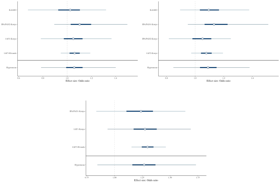
Figure I6: Bayesian Meta-analysis Effects (cont’d)
(a) Persistence (Lime) (b) Persistence (Fertilizers)
(c) Fatigue (Lime)
Notes: The figure plots the meta-analysis results for specific outcomes. The effects are estimated using Bayesian
hierarchical models. Results are reported in odds ratios. The horizontal lines denote 95% confidence intervals.
92

J Additional Program and Experiment Details
J.1 KALRO’s Program
The Kenya Agriculture and Livestock Research Organization (KALRO) is a public agency
with the mandate to promote agricultural research and dissemination in Kenya. In 2014 and
2015, KALRO’s Kakamega office implemented two extension programs designed to encour-
age smallholder farmers to use inputs and management practices that could remedy certain
regional soil deficiencies. The purpose of these programs was to reach many farmers at a
lower cost than in-person individual extension farm visits. The first program consisted of
one-day face-to-face events (farmer field days or FFDs) where many farmers could observe
demonstration plots and receive information from extension agents in a group setting. The
second program consisted of delivering agricultural messages to farmers via text messages.
This paper focuses on the results of the second approach.
35
KALRO’s text-message program consisted of sending 21 agriculture-related text messages
to maize farmers’ mobile phones during the 2015 short rains season. The content of the mes-
sages was developed by the Ministry of Agriculture, Livestock and Fisheries, while KALRO
managed the delivery. We list all messages sent by KALRO below:
• We at KALRO- Kakamega shall be sending
you 20 SMS tips on how to increase your
maize and legume (beans, groundnuts, soy-
beans) yield
• Keep all the records of your farming activi-
ties including inputs and outputs to help you
know whether your farming is profitable
• Test your soil after every 4 years. In-
quiries: KALRO Tel:[phone] or Soil Cares Ltd:
[phone]
• If soil is acidic (pH less than 5.5), apply rec-
ommended rate of agricultural lime at least 30
days before planting. Inquiries: Tel.[phone]
• Construct raised bands and trenches to con-
trol soil erosion, reduce nutrient loss and keep
rain water in the soil
• Add and/or leave all organic matter (manure,
crop/weed residues and compost) to your
field. Do not burn your fields. Burning de-
stroys useful micro-organisms.
• Prepare land early, at least one plough and
one harrow, ready for planting before onset
of rains
• Plant before or at the onset of rains. Plant on
well drained, fertile soils
• Use certified maize and legume seed recom-
mended for your area, bought from an ap-
proved agro-dealer. Use 10 kg maize seed
and 40kg of legume seed per acre. Inquiries:
[phone]
• Maize and legumes planted in rows are eas-
ier to weed & apply fertilizer. You may plant
maize alone/pure or together with legumes
as follows:
• For pure maize make rows 2.5 feet (75cm)
apart and holes 1 foot (30cm) apart along the
row. Place 2 and 1 maize seeds in alternate
holes.
• For maize and legume intercrop, plant maize
as for pure stand and one row of legume
(beans, soybean or groundnut) between two
maize rows at spacing of 10cm from one hole
to another.
• For better maize and legume harvests, inoc-
ulate legumes, rotate or intercrop, use fertil-
izer and manage your crop and soils appro-
priately.
• Use fertilizer to increases yields. Apply 1
heaped Fanta top of NPK or DAP in each
hole for maize, cover with little soil, add seed
and cover seed with soil. Fertilizer MUST not
touch the seed
• Weeds compete with your crops for nutrients
and so reduce yields. Keep fields free of
weeds and pests. Thin maize seedlings to 1
plant per hole as you weed.
• Topdress your maize with a level Fanta bottle
top of CAN or Mavuno top dress fertilizers
6 weeks after planting. Apply around each
plant-5cm away and cover with soil. Apply
when soil is moist.
• Harvest as soon as the crops are mature. For
maize look for the black eye; for legumes
when 90-100% of pods are brown. In late
harvests, termites, rodents, insects, diseases &
birds reduce yield.
• Remove husk from maize cobs in the field to
avoid transporting weevils from the field to
the store. The husks will improve the organic
matter in the soil.
• Dry your harvest in open sun, but protect it
from rain. Thresh/shell and re-dry to mois-
ture content of 11-12%.
• Store your harvest well in silos and helmetic
bags. You may also use superactellic during
storage – the insects will not touch the grain
& is safe.
• Obtain information on favorable market
prices before you sell your harvest
To recruit farmers into these programs, the evaluation team from IPA undertook a census
35
We discuss further details of the impacts of FFDs in Fabregas et al. (2017a).
93
of farmers residing in the Ugenya and Mumias sub-counties. The team employed a system-
atic approach, employing a set of predefined walking rules to visit a representative sample of
households in the selected areas. To identify eligible participants, farmers were required to
meet certain criteria, namely owning a mobile phone, having cultivated maize or legumes in
the previous year, and being responsible for farming activities within their households. Enu-
merators completed a total of 1,330 census surveys, and approximately 94% of those recruited
during census activities met the selection criteria.
In September 2014, farmers completed an in-person baseline survey and were then ran-
domized into the text-message (SMS) treatment (415 farmers) or a comparison group (417
farmers). The randomization was stratified on the basis of area of recruitment, gender,
whether farmers had heard about lime, an index of input use (divided into terciles), farm
size (above or below median), whether farmers grew legumes, and a cognitive score based on
a raven test and a math questionnaire (terciles).
The text-message service started in July and ended in November. An in-person endline
survey, asking information about input use and knowledge, was completed with 93% of the
baseline sample at the end of the season, around January 2016. Additionally, at the end of
the endline survey, all farmers received two physical (paper) discount coupons redeemable at
selected agricultural supply dealers in their nearest market center.
The coupons were devised as a way to collect data on farmers’ input choices while min-
imizing potential biases caused by enumerator demand effects, as farmers’ purchasing deci-
sions were postponed to a later time when they were not directly observed by any member of
the research or KALRO teams. The first discount coupon was redeemable for a 50% discount
for agricultural lime. The second coupon was redeemable for a 50% discount for any chemical
fertilizer of their choice (NPK, DAP, CAN, urea or Mavuno). Both coupons had an upper limit
discount of 1000 Ksh (approximately $10 USD). Coupon redemption was possible up to the
start of the subsequent long rain agricultural season (around March 2016). Participating agri-
cultural supply dealers were instructed (and incentivized through a small payment) to keep
clear records on input choices and quantities purchased by farmers who redeemed coupons.
Coupons could be linked to farmers through unique IDs. Incentives for shopkeepers were
paid on the basis of having both the physical coupon and a record of the purchase in their
logbooks.
94

J.2 IPA & PxD’s Programs
PxD supported two agricultural extension research projects in western Kenya that were im-
plemented and evaluated with support from IPA.
J.2.1 Program 1 (IPA/PxD1-K)
Throughout the 2016 short rain agricultural season, IPA and PxD, sent farmers in western
Kenya text messages with information about agricultural inputs (including lime and chemical
fertilizers), as well as other general agronomic recommendations on maize farming. Farmers
who participated in this program were recruited through administrative farmer records of
a large agribusiness in the region (denoted MSC farmers) and from records of individuals
who had participated in previous IPA’s activities (denoted IPA farmers).
36
In July 2016, a
random sample of farmers from both databases was contacted over the phone to invite them
to participate in this study and complete a short phone-based screening survey to determine
eligibility. Farmers who were planning to plant maize in the 2016 short rains season, had a
farm located within the intervention areas, and expressed interest in receiving agricultural
information over their phone were invited to participate. From 2,255 targeted respondents,
2,131 consented to participate, and 1,897 (89%) met the criteria for selection.
This final sample was randomized into three groups: receiving the general messages
(“General”), receiving specific messages for their area (“Specific”), and a control group. The
randomization was stratified based on database origin, area, gender, prior lime and urea use,
a knowledge score (below or above median), farm size (divided in terciles), whether they had
indicated a positive willingness to pay for the messages and whether they had replied to a
phone-based poll at baseline.
Customized recommendations used the best available soil data for each area. Farmers
received between 24 and 28 messages. Messages were sent in English or Swahili, depending on
farmers’ preferences indicated during the baseline phone survey. We report all the messages
below: [G] indicates that the message was received by the General treatment group, and [S]
denotes it was received by the Specific treatment group.
36
The Mumias Sugar Company (MSC) ran a contract farming model with sugar cane farmers in the region up
to 2015. The vast majority of MSC farmers planted maize in addition to sugar cane, so the company supported
the delivery of maize extension messages. The farmers who appeared in the IPA database were mainly recruited
through school meetings for other IPA projects. This group accounted for about 47% of the final sample.
95
• [G/S]: Welcome to PxD’s SMS information
service. We will give you tips on agricultural
inputs to apply on 1/8 of an acre so you can
experiment during this short rains season. Re-
ceiving SMS messages is free.
• [G]: High soil acidity levels reduce nutri-
ents available to plants, such as phosphorus,
which causes symptoms of stunted growth
and purple colouration of maize.
• [S]: Previous soil tests of shambas around
[landmark] showed [degree] soil acidity lev-
els. High acidity levels reduce nutrients avail-
able to plants, such as phosphorus, which
causes symptoms of stunted growth and pur-
ple colouration of maize.
• [G]: Lime reduces soil acidity and makes nu-
trients such as phosphorus available for your
maize.
• [S]: Based on soil tests of shambas around
[landmark], we recommend you buy [quan-
tity] kg of lime, [quantity] kg of DAP, and 6
kg of urea for microdosing 1/8 acre of your
maize. Lime reduces soil acidity and makes
phosphorus available for your maize.
• [S]: We would like you to try our recommen-
dations in 1/8 of an acre. To measure 1/8 of
an acre, walk around your farm and draw a
square with each side 33 steps long. Walk nor-
mally, don’t make long strides. If you land is a
rectangle, the sum of 2 sides should measure
in total 66 steps. Start from a corner, walk
along the short side, count your steps until
you reach the end. Turn around and keep
walking along the long side until you finish
counting 66 steps.
• [S]: When planting this season try adding a
layer of lime [quantity] bottletop, then cover
with soil and add a second layer of DAP
([quantity] bottletop) per hole on 1/8 acre to
correct soil acidity and make more nutrients
available for your plants. Apply 1 bottletop of
urea per hole at top dressing.
• [G]: Use a ruler or measured rope to plant
maize in rows using correct spacing of 75 cm
x 25 cm. This offers maximum yield while
limiting competition for nutrients, light and
water.
• [S]: Use a ruler or measured rope to plant
maize in rows using correct spacing of 75 cm
x 25 cm. This offers maximum yield while
limiting competition for nutrients, light, and
water. You should be able to fit 2580 planting
holes in 1/8 of an acre. Use sisal twine to en-
circle this area so you can compare the results
at harvest.
• [S]: Have you bought lime and DAP yet? If
not, buy a total of [quantity] kg of lime and
use with [quantity] kg DAP for microdosing
on 1/8 of your acre. DAP is the most cost
efficient source of phosphorous. When lime
is combined with DAP, it reduces soil acidity
and makes nutrients available for your maize.
• [G]: Calcium lime is safer for your health and
the plant. This lime could be either brown or
grey.
• [S]: [agrovet] will be stocked with lime (cal-
cium lime) and DAP during this short rain
season. This lime is brown and it is safer for
your health and the plant. It is also heavier
than the white lime so you only need to ap-
ply [quantity] bottletop per plant. The price
of lime today is Ksh 7 per kg. The price of
DAP today is Ksh [price] per kg.
• [G/S]: Plant maize seed when there is enough
moisture after 2-3 rains, to enable absorption
of water by seed and fertilizer. Delayed plant-
ing leads to reduced yields. To stop receiving
these SMS messages reply ”STOP”.
• [G/S]: Plant two maize seeds per hole to en-
sure one survives. Do not use broken or dam-
aged seeds because they will not germinate.
Use certified seeds, they grow faster and are
high yielding.
• [G]: Are you ready to plant your maize? We
recommend you apply both lime and fertilizer
in micro-doses at planting. 5 weeks later, we
recommend you apply top dressing fertilizer
in micro-doses
• [S]: Do you know the 5 Golden Rules for suc-
cessful micro-dosing? Based on soil tests per-
formed around [landmark], we recommend
you to: Apply [quantity] bottletop of lime and
cover with soil and then add [quantity] bottle-
top of DAP. Cover with 2 inches of soil. Use
2 seeds per planting hole. Cover the seeds
with 2 inches of loose soil. Apply 1 bottletop
of urea as top dressing fertilizer 5 weeks later
when the plant is knee-high.
• [G/S]: Remember, lime should only be used
during planting and not at top dressing. Lime
is not a fertilizer and could burn the plant if
applied at top dressing.
• [G/S]: At planting, if you are applying lime
in micro-doses, remember to cover it with soil
before applying fertilizer and planting seeds.
Lime should not be in direct contact with the
seeds as it may burn them. When you apply
lime, wear protective clothing such as long
sleeves and gloves. Cover your mouth and
nose with a scarf and wear goggles.
• [G/S]: Gap your maize immediately after
emergence. Gapping is done by re-planting
maize seeds in places that have not germi-
nated. This gives you optimum plant popu-
lation that leads to optimum yields.
• [G/S]: During first weeding, thin to one maize
plant per hole. You should remove striga im-
mediately to reduce competition for nutrients
and water, and to prevent stunted growth!
• [G]: Have you already planted your maize this
season? If not, we recommend applying lime
at planting. Lime reduces soil acidity and
makes nutrients such as phosphorus available
for your maize.
• [S]: Have you already planted your maize this
season? If not, we recommend applying lime
at planting. We recommend you apply [quan-
tity] bottletop per planting hole. Buy [quan-
tity] kg of lime to experiment on 1/8 of an
acre. Lime reduces soil acidity and makes nu-
trients such as phosphorus available for your
maize.
• [G]: If you applied lime on your maize at
planting, we recommend using urea at top
dressing because it is a less expensive source
of nitrogen.
• [S]: If you applied lime on your maize at
planting, we recommend using urea for top
dressing because it is a less expensive source
of nitrogen. Buy 6 kg of urea for use on 1/8
of an acre.
• [S]: [agrovet] will be stocked with urea during
this short rain season. The price of urea is Ksh
[agrovet] per kg.
• [G]: When the maize reaches knee high (5
weeks after planting), apply top dressing fer-
tilizer.
• [S]: When the maize reaches knee high(5
weeks after planting), based on soil tests
around [landmark], we recommend you ap-
ply 1/2 bottletop of urea per plant, making a
15 cm circle around the maize plant.
• [G/S]: Conduct second weeding 6 or 7 weeks
after planting. Uproot all striga before it pro-
duces seeds because it reduces maize yields if
not removed
• [G/S]: We invite you to participate in an SMS
poll to help you recognize potential maize dis-
eases and provide advice. Reply OK to start.
Messages are free.
– Do you see straight lines of holes on
newly formed maize leaves?
[if yes] This could be stalk borers.
Apply insecticide, e.g. bulldock or
tremor, into the funnel or spay the
maize plant with pentagon at top
dressing.We hope this information
was helpful. We will be sending an-
other poll question tomorrow. Thank
you!
[if no] This is good news! Thank you
for answering our question. We will
send another question tomorrow.
– Do you notice yellow or white
streaks or discoloration on the leaves
of your stunted maize plants? [if yes]
It could be Maize Streak Virus. Erad-
icate grass weeds and use malathion
or dimethoate to control as soon as
possible. We hope this information
was helpful. We will be sending an-
other poll question tomorrow. Thank
you!
[if no] This is good news! Thank you
for answering our question. We will
send another question tomorrow.
– Do you see striga weed in your
maize plot? Striga has thin leaves
and pink or purple flowers and at-
taches onto the maize roots.
[if yes] Uproot all striga that has
emerged. Striga competes with your
maize for nutrients, water, and light
and leads to reduced maize yields.
We hope this information was help-
ful. We will be sending another poll
question tomorrow. Thank you!
[if no] This is good news! Thank you
for answering our question. We will
send another question tomorrow.
– Do you see ants that cut maize stalks
and feed on fallen maize cobs?
[if yes] It could be termites. Dig
out all anthills around your maize
farm and ensure that you destroy the
queen. Alternatively, you can dig a
deep hole at the center of the anthill
and use insecticide to kill the ants.
We hope this information was help-
ful. This is the last poll question. We
will NOT send another question to-
morrow. Thank you for your partici-
pation!
[if no] This is good news! This is the
last poll question. We will NOT send
another question tomorrow. Thank
you for your participation!
• [G/S]: WEEDING REMINDER! Conduct sec-
ond weeding 6 or 7 weeks after planting.
Weeds compete with your maize for nutrients,
water, and light, which reduces yields.
• [G]: Have you already applied top dressing
fertilizer on your maize? If not, we recom-
mend using urea at top dressing because it is
a less expensive source of nitrogen.
• [S]:Have you already applied top dressing fer-
tilizer on your maize? If not, we recommend
using urea at top dressing because it is a less
expensive source of nitrogen. Buy 6 kg of urea
for use on 1/8 of an acre and apply 1/2 bottle-
top of urea per plant. Apply urea when there
is enough moisture in the soil to avoid loss
through evaporation.
• [G/S]: Harvest maize at physiological matu-
rity when cobs droop and leaves dry. Dry
maize in the sun even after shelling to avoid
mold and attack by weevils. Maize grain must
remain dry and clean during storage to avoid
reduction in quantity and quality.
• [G/S]: We hope you enjoyed these messages
from Precision Agriculture for Development.
Our team will follow up with a phone call
in the coming weeks to hear more about how
your planting season went.
96
Two electronic discount coupons were sent via text message to all participating farmers,
including those in the control group, during the short rains 2016. Farmers could redeem
coupons in agricultural supply dealers in their preferred or closest market center (selected
by farmers during baseline). The first coupon was sent ten days after the beginning of the
experiment, after seven recommendation messages, with a reminder one week later. The first
coupon gave farmers a choice of either 10 kg of lime or 1 bar of soap. The purpose of allowing
farmers to select between lime and another comparable product of equal value was to capture
farmers’ input preferences free from other liquidity constraints.
The second coupon was sent one month after the beginning of the experiment, after 18
messages, with a reminder after ten days and another 20 days later. This coupon provided
a 30% discount on one type of top-dressing fertilizer (urea, CAN, or Mavuno), up to a pre-
discount amount of 500 Ksh (approximately $ 5 USD).
Additionally, during the 2017 long rains season, all treated farmers received five identical
text messages about agricultural lime:
• [If pH≤5.5]: The soil in your area is [level] acidic. To avoid low yields,
treat now. Apply [quantity] bottletop of lime per planting hole. [quantity]
lime per 1/4 acre.
• [If pH>5.5]: The soil in your area is slightly acidic. According to our
analysis, farms in your area do not need lime.
A phone endline survey was conducted mid-2017 long rain season, with the full sample
of farmers participating in the experiment. The survey included questions about input use
during the 2016 short rain and 2017 long rain agricultural seasons, as well as farmers’ general
agricultural knowledge. Enumerators completed surveys with approximately 80% of farmers
in the sample.
J.2.2 IPA/PxD2-K
The second IPA/PxD program recruited farmers through agricultural supply dealers. A total
of 144 agricultural supply dealers in 60 market centers invited farmers to provide their phone
numbers if they were potentially interested in participating in an IPA/PxD program. The
registration period ran from early December 2016 to late January 2017. A total of 8,496 farmers
were registered.For logistical reasons, the study area was later restricted to 46 market centers,
which contained 102 agricultural supply dealers. Farmers in these centers were then contacted
over the phone by a member of the research team to obtain consent and to complete a baseline
97

survey, which contained questions about their farming practices and previous input use. A
total of 5,890 farmers completed the phone baseline survey, met the eligibility criteria, and
resided in eligible areas for which PxD had soil information.
37
Farmers were then randomized into four groups. The first three groups received PxD’s
text message information services, and the fourth group remained as a control. One-third
of treated farmers received information via SMS only, another third received SMS and were
invited to express interest in receiving a phone call that would explain the messages, and the
last third of treated farmers were directly contacted over the phone and offered an explanation
of the messages. The randomization was stratified by gender, prior lime use, and by the
agrovet that recruited the farmers.
Messages were sent during the 2017 long rains season and were based on ward-level soil
test data. Wards were chosen because they are one of the smallest units that farmers can
self-report and that soil tests could be mapped into.
38
The messages focused on three types of recommendations: the use of agricultural lime in
wards with median soil pH below 5.5, the use of planting fertilizer, and the use of top-dressing
fertilizers, primarily urea. Messages were sent in either English or in Swahili, depending on
farmers’ language preferences at the time of registration. We list them below [A] indicates
that all treated groups received the message, and [SCO] denotes it was received by the ‘SMS
+ Call Offer’ group. In addition to these messages, the ‘SMS+ Call’ [SC] group received a
call from an extension officer to explain these messages. This 15-minute phone call did not
provide any additional information, but it allowed farmers to ask clarification questions to a
PxD field officer and to hear the explanation multiple times. The purpose of the phone call
was to strengthen the information provided via text.
• [A] Welcome to PxD, IPA’s free advice service
for maize growers. You will receive advice
for your needs based on more than 10,000 soil
tests from western Kenya.
• [A] The soil in your area is [level] acidic. To
avoid low yields treat now. Apply [quantity]
bottle top of lime per planting hole. [quantity]
kgs for 1/4 acre. OR The soil in your area is
slightly acidic. According to the soil analysis,
farms in your area do not need lime.
• [A] Soil acidity causes stunted growth. Lime
reduces soil acidity and makes nutrients of
DAP more available for your maize.
• [A] When planting, apply [quantity] bottle
top of lime. Cover with a handful of soil.
Add [quantity] bottletop of DAP, cover with
enough soil to avoid direct contact of inputs.
OR When planting, apply [quantity] bottle
top of DAP, cover with enough soil to avoid
direct contact of inputs.
• [A] Check your phone! We sent you 3 plant-
ing recommendations last week./ [if SCO] If
you flash [number] before Friday this week,
we will you callback soon to explain them/ [iF
SCO] We will call you soon to explain them]
• [A] Top-dress when your maize has more than
4 leaves up to knee-high. If rains are good ap-
ply [quantity] bottle top of UREA. If rains are
low, apply [quantity] bottle top of CAN.
• [A] UREA can increase your maize yields as
much as CAN if rains are good. Try [quantity]
kg of urea in 1/4 acre and see the results.
• [A] Check your phone! We sent you 2 top-
dressing messages this week./[if SCO] If you
reply YES or flash [phone] by Tuesday, we will
call you back soon to explain them./ [if SC]
We will call you soon to explain them.
37
From the original sample, farmers who were reached but did not complete the baseline survey included 257
who did not consent to participate in the study, 53 who were not planning to grow maize in 2017, and 40 who
lived outside the four counties in which recruitment took place. Approximately 1,017 farmers lived in wards for
which there was no soil test data available.
38
In western Kenya, the average size of a ward is 12 km
2
.
98

All farmers participating in the experiment received two electronic coupons via text mes-
sage. Each coupon allowed farmers to obtain discounts on agricultural inputs from a local
agricultural supply dealer. The first electronic coupon was redeemable for 15% on the first
seven 10-kg bags of agricultural lime, and the second coupon provided a 15% discount on
the first 1,000 Ksh (approximately $10 USD) spent on top-dressing fertilizers (urea, CAN, or
Mavuno). To ensure that all farmers in the treatment and control groups were equally aware
of the coupon, all farmers received a phone call a week before the coupon was sent, in which
an enumerator explained how to use the coupon and at which agricultural supply dealers the
coupons could be redeemed. 93% of farmers were reached during this activity.
Finally, a phone-based endline survey was completed with this sample. Because of logis-
tical constraints, the survey sample was randomized into two groups: completing the survey
early (towards the end of the 2017 long rains) or completing the survey late (towards the end
of the 2017 short rain season). Of those who completed the survey, 33% completed it early,
and 67% completed it late. In total, 84% of the initial sample completed the survey.
Both versions of the survey included questions regarding the farmers’ agricultural knowl-
edge and input use during the 2017 long rain season. Additionally, the late survey had ques-
tions about input usage during the 2017 short rain season. To measure the persistence of input
use over the subsequent season, we use usage data obtained from the subsample of farmers
who were randomly assigned to complete this portion of the survey.
J.3 One Acre Fund’s Programs
1AF operates in six countries in Eastern and Southern Africa. In 2017, they were working
with over 600,000 farmer clients (1AF, 2017). The standard bundle that 1AF offers includes
hybrid seeds and chemical fertilizers. However, to address the problem of high soil acidity,
1AF offered farmers agricultural lime as an optional add-on. Yet, across their many locations,
demand for lime remained low. Hypothesizing that this could reflect a lack of awareness,
1AF designed and evaluated several informational programs to increase lime take-up. Since
1AF field officers already follow detailed protocols, a key objective of the approach was to
test cheap programs that would not require additional field officer training and delivery. We
describe 1AF’s different strategies below.
99
J.3.1 1AF1-K
Before 2016, less than 3% of 1AF clients in western Kenya purchased agricultural lime through
the organization (1AF, 2015). To increase take-up, 1AF designed a phone-based extension pilot
that consisted of six text messages targeting clients who had signed up for the 1AF package
during the previous season in a selected district of western Kenya.
In September 2016, during the period in which 1AF farmers were placing their orders for
the 2017 long rains season, 1AF sent text messages about soil acidity and agricultural lime.
Two types of messages were sent: the first, denoted as “Broad”, simply encouraged farmers
to use lime to reduce soil acidity and increase yields, while the second, denoted as “Detailed”
provided recommendations on lime application rates and expected yield increase, customized
to the farmers’ site. Customized messages were based on soil tests that had been previously
conducted by 1AF in the region. In total, 4,884 farmers participated, with 3,325 randomly
assigned to receive messages and 1,559 remaining as a control. The same SMS message was
sent six times between August and September 2016, before the 1AF input contract signing
period, when farmers had to decide whether to request inputs from 1AF for the following
season (long rains 2017).
Farmers in both treatment groups received six identical messages, all messages were sent
in Swahili. We report the messages below:
• [Broad]: Hello [name],Your soil is acidic. Use lime to reduce acidity and
increase yields.Call xxx-xxxx.
• [Detailed]: Hello [name],Your soil is [level] acidic. We recommend
[amount] kg of LIME per acre at [total cost] Ksh. Use lime to reduce acidity
and increase yields [percentage increase]%.Call xxx-xxx.
To measure outcomes, we use two sources of data: 1AF administrative data and phone
survey data collected with a random subsample of farmers. The administrative data includes
details on loan enrollment and inputs purchased through the 1AF program for the 2017 and
2018 long rain seasons. However, it is important to note that only around 60% of the farm-
ers who received the text messages later registered for 1AF loans during the 2017 long rain
agricultural season. Therefore, input purchases from the administrative data are conditional
on enrolling in the 1AF program that season. We take a conservative approach and define
our main outcome as lime purchases acquired through 1AF (coding as zero those who never
enrolled). However, we also show effects conditioning on the 2017 1AF enrollment (we find
no evidence that messages affected the likelihood of being enrolled in the 1AF program).
100
To gather more information from farmers, IPA conducted a follow-up phone survey in
May 2017 with a random subsample of 30% of the experiment’s farmers. This survey asked
respondents about their lime knowledge and input use during the 2017 long rain season.
Approximately 79% of the contacted farmers completed the survey.
In September 2017, at the time of enrollment for the 2018 long rains season, farmers in
the experiment who had also enrolled in the 1AF program for the 2017 long rains season
were re-randomized into receiving additional messages about lime. A total of 2,931 farmers
were re-randomized, essentially resulting in the creation of four groups: farmers who never
received messages, farmers who received messages during two seasons, farmers who were
only treated just before the 2017 season, and farmers who were only treated just before the
2018 season. They received the following message one to five times:
• 1AF recommends you register to buy lime for your maize.
Outcomes for this season are also measured through 1AF administrative records.
J.3.2 1AF2-K
A second 1AF program was implemented with approximately 30,000 farmers in four Kenyan
districts in September 2017. Former 1AF clients were randomized into a no message control
group or a treatment group receiving SMS messages encouraging lime adoption. Additionally,
a quarter of farmers were randomly assigned to receive additional messages encouraging
additional fertilizer use (extra CAN) for top-dressing.
Six different types of messages were sent: a “Basic” message simply recommending pur-
chasing lime, a message, “Yield increase”, also mentioned that lime would increase yields, two
encouraged experimentation, “Experimentation (selfish)” and “Experimentation (neighbors)”,
and two leveraged on behavioral nudges “Social comparison” and “Self-efficacy”. Half of
the treated farmers were randomly assigned to receive messages addressing the whole family
instead of the individual (by replacing the word “you” with “your family”). The messages
encouraging use of additional quantities were identical to those encouraging use of lime (the
word “Lime” was replaced by “Extra CAN”). Farmers assigned to receive both lime and fer-
tilizer messages were randomly assigned to receive one of the two first and the other on the
next day for all repetitions. The number of repetitions (from 1 to 5) were cross-randomized.
101
In September 2018, at the time of enrollment for the 2019 long rains season, all the farmers
who purchased inputs from 1AF for the 2018 long rains season received additional messages
encouraging lime adoption (but no messages about fertilizer). We report messages below:
• [M1: Basic] [Name], 1AF recommends
[you/your family] register to buy
[Lime/Extra CAN] for your maize.
• [M2: Yield increase] [Name], 1AF recom-
mends [you/your family] register to buy
[Lime/Extra CAN] for your maize. You’ll get
higher yields by using [Lime/Extra CAN].
• [M3: Experimentation (selfish)] [Name], 1AF
recommends [you/your family] register to
buy [Lime/Extra CAN] for your maize. Try
it on just a small part of your land to see the
benefits.
• [M4: Experimentation (neighbors)] [Name],
1AF recommends [you/your family] register
to buy [Lime/Extra CAN] for your maize. Try
it on just a small part of your land to so that
you and your neighbors can see the benefits.
• [M5: Social Comparison] [Name], 1AF rec-
ommends [you/your family] register to buy
[Lime/Extra CAN] for your maize. Farmers
all over western are getting bigger yields by
using [Lime/Extra CAN]. Keep up with them!
• [M6: Self-efficacy] [Name], 1AF recom-
mends [you/your family] register to buy
[Lime/Extra CAN] for your maize. You have
the ability to achieve higher yields by using
[Lime/Extra CAN]!
Farmers were later matched to 1AF administrative data to measure their likelihood of
demanding agricultural lime and other inputs for the following two agricultural seasons.
J.3.3 1AF3-R
In Rwanda, 1AF, locally known as Tubura, had established a partnership with the government
aimed at providing farmers in the region with access to agricultural products, services, and
training. Since 2016, they had been collaborating to promote the widespread adoption of
agricultural lime.
In 2017, 1AF introduced a text-message-based program designed to encourage farmers to
experiment with a specific type of agricultural lime called travertine.
Similar to 1AF2-K, the evaluation aimed to assess the impact of messages and identify the
most effective message framing and frequency by introducing randomization within the pro-
gram. Additionally, due to the relatively low mobile phone penetration in the country, 1AF
sought to investigate potential spillover effects within farmers’ groups. To capture this, ran-
domization was implemented at both the group and individual levels. Initially, farmer groups
were randomly assigned to one of three categories: a pure control group, where no farmers
received messages; a pure treatment group, where all farmers with phones received messages;
and a partially treated group, where farmers with phones had a 50% chance of receiving the
message. The content and frequency of these messages (ranging from 1 to 5 repetitions) were
randomized at the individual level. The message framing variations included:
• [T1-G: General promotion (gain)] Many
fields in Rwanda have acidic soil and need
TRAVERTINE to increase yields. Order from
TUBURA now.
• [T1-L: General promotion (loss)] Many fields
in Rwanda have acidic soil and need
TRAVERTINE to avoid a yield loss. Order
from TUBURA now.
• [T2-G: Specific+ yield impact (gain)] Many
fields in Rwanda have acidic soil. Applying 25
kg/are of TRAVERTINE will increase yields
by 20%.Order from TUBURA now.
102
• [T2-L: Specific+ yield impact (gain)] Many
fields in Rwanda have acidic soil. Applying 25
kg/are of TRAVERTINE will prevent a yield
loss of 20%. Order from TUBURA now.
• [T3-G: Self-diagnosis (gain)] Do you have
fields with poor harvests even when you use
fertilizer? You probably have acidity and need
TRAVERTINE to increase yields. Order from
TUBURA now.
• [T3-L: Self-diagnosis (loss)] Do you have fields
with poor harvests even when you use fer-
tilizer? You probably have acidity and need
TRAVERTINE to avoid a yield loss. Order
from TUBURA now.
• [T4-G: Soil test (gain)] Ask your Field Officer
for a free soil test to learn if your fields are
acidic and you need to order TRAVERTINE
to increase yields.
• [T4-L: Soil test (loss)] Ask your Field Officer
for a free soil test to learn if your fields are
acidic and you need to order TRAVERTINE
to avoid a yield loss.
• [T5-G: How travertine works (gain)] Many
fields in Rwanda have acidity, which blocks
fertilizer uptake. Applying TRAVERTINE
solves the problem, increasing crop yields.
Order from TUBURA now.
• [T5-L: How travertine works (loss)] Many
fields in Rwanda have acidity, which blocks
fertilizer uptake. Applying TRAVERTINE
solves the problem, preventing a yield loss.
Order from TUBURA now.
• [T6-G: Order immediately (gain)] Many
fields in Rwanda have acidic soil and need
TRAVERTINE to increase yields. Order it im-
mediately, when signing your TUBURA order
form.
• [T6-L: Order immediately (loss)] Many fields
in Rwanda have acidic soil and need
TRAVERTINE to avoid a yield loss. Order it
immediately, when signing your TUBURA or-
der form.
• [T7-G: Your cell is acidic + yield impact (gain)]
In your cell the soil is acidic. If you apply 25
kg/are of TRAVERTINE you can boost yields
by 20%. Order from TUBURA now.
• [T7-L: Your cell is acidic + yield impact (loss)]
In your cell the soil is acidic. If you apply 25
kg/are of TRAVERTINE you can avoid a yield
loss of 20]%. Order from TUBURA now.
From a total of 202,972 farmers registered in the 1AF program, 110,400 had a phone reg-
istered in the 1AF database. As an outcome measure for the first season, we use whether
farmers purchased lime from 1AF in the 2018 agricultural season (about 62% of farmers who
received messages, enrolled in the 1AF loan program during that season agricultural season
and were eligible to buy lime). In the main analysis, we compare farmers from the fully treated
and pure control farmer groups and exclude those from partly treated groups (including the
partly treated groups does not change the results).
During the second season, farmers who had enrolled in the 1AF program in 2018 were
re-randomized at the group level to receive the messages below. Within groups assigned to
treatment, messages were further randomized at the individual level. This effectively created
three types of treatment assignments: those farmers who never received messages, those who
received messages during two seasons, and those who received messages only during the first
or second season.
• [M1: Basic Message] Hi [Name], use traver-
tine, fertilizer and compost on your fields this
season to get a better harvest. Buy travertine
and fertilizer from Tubura!
• [M2: Feed your family] Hi [Name], use traver-
tine, fertilizer and compost on your field this
season. You’ll get better harvests to feed
your family. Buy travertine and fertilizer from
Tubura!
• [M3: Social comparisons] Hi [Name], some
Tubura farmers have doubled their harvest by
using travertine with fertilizer and compost.
Buy travertine and fertilizer from Tubura!
• [M4: House metaphor] Hi [Name], to get
great harvests, you build your soil’s strength
like you build a house. Compost is the foun-
dation, travertine is the strong frame, and fer-
tilizer is the roof. Buy travertine and fertilizer
from Tubura!
During this season, 66% of those who were re-randomized re-enrolled in the 1AF program
and were, therefore, eligible to order lime during the second season.
103
K Agricultural Recommendations
In this section, we first describe how the agronomic recommendations were constructed. We
then discuss how informative area-level recommendations might have been for individual
farmers, and the potential for errors of inclusion.
K.1 Generating Agricultural Recommendations
KALRO. Officials and extensionists from KALRO and the Ministry of Agriculture developed
the content of the messages. The recommendations were crafted based on the officials’ knowl-
edge of broad agro-ecological zones and the types of soils in western Kenya. KALRO classifies
all the regions where they worked as having acidic soils (Kanyanjua et al., 2002), but farmers
were advised to test their own soil and use the recommended amount of lime resulting from
those tests.
IPA-K/PxD1-K. Recommendations were crafted by agronomists based on available soil data.
All farmers were linked to a nearby identifiable landmark with associated soil data. This
approach was necessary due to the absence of consistent village names or addresses in this
context. Farmers recruited through the IPA database were matched to their closest primary
school and were provided with recommendations based on soil tests performed around these
schools (the vast majority were within 1 km of the landmark and almost all within 2 km).
Soil data for these recommendations was previously collected for other IPA projects in 2011
and 2014 (Fabregas et al., 2017b) and analyzed by the Kenya Agricultural Research Institute
(KARI) using wet chemistry. Lime quantities were calculated based on the standard lime
factor of 1.5 times the exchangeable acidity (Kamprath, 1970). Farmers recruited through the
MSC database were already assigned to a specific ‘company field’, a set of plots cultivated
by multiple farmers and aggregated by the company for conducting activities, including soil
testing. Lime recommendations were based on median pH, with those in areas with a median
pH over 5.5 not receiving lime messages. Among both these samples, approximately 18% did
not receive messages about lime.
Farmers also received messages about planting (DAP) and top-dressing (urea) fertilizers.
The amount of planting fertilizer recommended was based on the median amount of phos-
phorus measured in the area, which determined the recommended quantity of diammonium
104
phosphate (DAP).
Top-dressing fertilizer recommendations were based on the quantity of nitrogen required
to achieve a certain expected yield. The quantity was selected based on the target yield of
2 t/ha, which is standard for the area. Urea was recommended, given that it was a cheaper
source of nitrogen.
IPA-K/PxD2-K. Farmers participating in this study were provided with lime recommenda-
tions based on the median soil pH in their ward. Only those with median pH below 5.5 were
recommended to lime (77% of the sample). Planting fertilizer (DAP) recommendations were
based on median values of phosphorous. The recommended DAP quantities were based on a
target yield of 2 t/ha, which was chosen as it represented an improvement with respect to the
baseline average yield of 1.42 t/ha, while keeping the cost of the input package affordable for
the farmers.
Top-dressing fertilizer recommendations were based on the quantity of nitrogen required
to achieve a certain expected yield. As with the first project, the objective of the messages
was to encourage farmers to experiment with urea, a less commonly used fertilizer. Farmers
were advised to opt for urea if the rainfall conditions were good. While urea is a cheaper
source of nitrogen, its efficiency diminishes in dry conditions due to the potential for ammonia
volatilization. Messages mentioned CAN as an option for top-dressing if rain was low. Since
rains were considered good during this season, we take experimentation with urea as the
primary indicator of following recommendations. However, we also show impacts if either
CAN or Urea were used.
The ward level was used for recommendations because it was the most precise information
that could be used about farmers’ location and that soil data could be consistently linked to.
Soil data was pooled from four different sources: (i) Soil data collected by IPA-K in Busia
county for previous projects (Fabregas et al., 2017a) in 2011 and 2014 and as part of test plot
activities conducted in 2016, (ii) Soil data collected by 1AF across the entire study area in
2016, (iii) Soil data collected by Mumias Sugar Company in Busia and Kakamega counties
between 2009 and 2016, (iv) Soil data collected by the German Agro Action (Welthungerhilfe)
in Kakamega and Siaya counties in 2015. Data collected before 2014 was dropped if at least 30
more recent observations in the ward were available. The final soil test dataset used included
about 7,085 observations for 108 wards.
105
1AF1-K. The standard application rate recommended by 1AF and reflected in field materials
was 200kg/acre across the entire program. To generate “local” recommendations, 1AF’s used
their own soil tests, performed using soil spectroscopy, and soil data collected for a previous
project by IPA-K (Fabregas et al., 2017b) and analyzed by the Kenya Agricultural Research
Institute (KARI) using wet chemistry in 2011 and 2014. These soil chemistry results were then
interpolated across areas through kriging to create a continuous field of soil chemistry predic-
tions. Since 1AF does not collect the coordinates of farmers’ plots, farmers were assigned to
the GPS coordinates of the site to which inputs are delivered by 1AF.
Optimal lime application rates for each level of pH were based on 1AF on-farm agronomic
trials conducted in 2015 (1AF, 2015). During that trial three different lime application rates
were tested: 50kg/acre, 100kg/acre, and 200kg/acre. The sample was divided according
to pH quintiles and, for each quintile, the lime application rates that resulted in the most
precisely estimated effect on yield was chosen. Two different lime application rates were
recommended, based on the local predicted level of pH: 200kg/acre and 50kg/acre. For
additional information on 1AF recommendations and the krigging procedure, see: https:
//ond3.com/lime_sms.nb.html#site-level_ph_levels.
106

Figure K1: Soil Map of western Kenya
(a) Phosphorus
Notes: Panel (a) shows the median level of Phosphorus (P) in all wards in which the IPA/PxD2-K program took
place, as well as the location of the programs.
K.2 Considerations in Using Area-level Information to Generate Agricultural Ad-
vice
KALRO classifies the areas where the Kenyan projects took place as having moderate to ex-
treme soil acidity (Kanyanjua et al., 2002). A large fraction of Rwanda’s arable land is also
considered acidic (Nduwumuremyi et al., 2014). However, it is also expected that hetero-
geneity in soil characteristics will lead to differential returns to liming for individual farmers.
In particular, one consideration is the extent to which some farmers who received messages
about lime might not have needed to apply the input.
First, when turning to the data, the assumption that lime has no benefits for those with a
pH over 5.5 or 6 might be too strong. Using data from 1AF’s experimental lime plots in Kenya,
we find that, on average, liming increased maize yields even in farms that initially had pH
levels above 5.5 (Appendix Figure K2). This might be because of a measurement error in soil
tests or because micro-dosing lime can also make up for deficiencies of other micronutrients,
like calcium.
107

Figure K2: Impact of Liming on Maize yields by Soil pH (1AF Agricultural Trials)
Effect of lime - pH<5.5
Effect of lime - pH>5.5
-.5 -.3 -.1 .1 .3 .5 .7 .9
Effect on yield t/ha
Notes: The figure shows effects of lime on maize yields from over 1AF’s experimental lime plots implemented in
Kenya. The figure shows heterogeneity based on whether the plots had pH values under 5.5 or over 5.5 before
lime was applied.
However, even if one takes as given that a pH of 5.5, 6, or 7 is the true threshold for
benefiting from lime use, an important question is how much heterogeneity there was in
pH levels in the areas where lime was recommended. To speak to this issue, we use soil
information from over 8,193 soil tests conducted in Kenya and 2,534 conducted in Rwanda,
both from the regions where programs were implemented and lime was recommended. To
the extent that these soil tests are representative of the underlying distribution of pH among
farmers who took part in the programs, we can approximate the share of farmers who received
lime advice and whose soils were under standard acidity thresholds.
Table K1 columns (1)-(3) report a ‘naive’ estimate of the fraction of soil tests taken in areas
where programs recommended farmers to use lime, and that had pH levels under 5.5, 6, or 7.
The majority of tests are under the acidity thresholds.
These naive estimates, however, will tend to overestimate the share of outliers in the pH
distribution given measurement error in soil test measurement. Therefore, we adjust these
estimates to account for measurement errors in individual soil tests.
To see this, suppose that there are locations i=1,...,N. At each location, one can observe the
pH results from a soil sample tested twice q
im
, where m = 1, 2 denotes measurement 1 or 2.
The measurements of pH are noisy with iid errors:
q
im
= Q
i
+ e
im
, e
im
∼ N (0, σ
2
e
)
108

Q
i
is the true soil pH at location i and the object of interest for a farmer. With this set up,
we have that q
im
| Q
i
∼ N (Q
i
, σ
2
e
). The true pH is generated by:
Q
i
=
¯
Q + θ
i
, θ
i
∼ N (0, σ
2
θ
)
Knowing that the test-retest correlation, r, corresponds to:
r = corr(Q
i
+ e
i1
, Q
i
+ e
i2
)
=
cov(Q
i
+ e
i1
, Q
i
+ e
i2
)
p
var(Q
i
+ e
i1
) ∗ var(Q
i
+ e
i2
)
=
σ
2
θ
q
σ
2
θ
+ σ
2
e
1
∗
q
σ
2
θ
+ σ
2
e
2
We can then estimate σ
2
θ
to get the ‘true’ share of soil tests with pH below 5.5, 6 or 7. In
a sample of 563 soil tests blindly tested twice by the National Soil Laboratory in Kenya, we
estimate r to be 0.73 for soil pH. Assuming that this test-retest correlation is representative for
all soil tests in the sample, we can then estimate σ
2
θ
for all programs. With this correction, we
estimate that 97% of soils in the areas where lime was recommended were under a pH of 6
and 69% had a pH below 5.5 (Table K1 columns (5)-(7)).
Table K1: Share of acidic soil tests in areas where lime was recommended
Trial No. soil Naive share Adjusted share
tests pH<5.5 pH<6 pH<7 pH<5.5 pH<6 pH<7
(1) (2) (3) (4) (5) (6) (7)
KALRO 632 0.83 0.98 0.99 0.87 1.00 1.00
IPA/PxD1-K 2799 0.77 0.95 1.00 0.82 1.00 1.00
IPA/PxD2-K 6234 0.77 0.95 1.00 0.81 0.99 1.00
1AF1-K 703 0.78 0.97 1.00 0.86 1.00 1.00
1AF2-K 4186 0.77 0.94 1.00 0.80 0.99 1.00
1AF3-R 2318 0.51 0.77 0.99 0.51 0.86 1.00
Pooled Sample 9213 0.68 0.90 1.00 0.69 0.97 1.00
Notes: KALRO recommended farmers to use lime only after testing their own soil. Soil tests can
overlap between different trials. In total, projects had access to data from 8,061 soil tests in Kenya and
2,318 in Rwanda. The source of all soil test data is discussed in Appendix section K.1.
We also assess what the differential costs of realizing low returns from lime would have
been between those in the treatment and control groups. One natural hesitation in providing
109
farmers information about lime is that if too much is applied, it could make soil pH levels
alkaline. In the context of these experiments, which mostly recommended microdosing rather
than broadcasting, this was highly unlikely. A meta-analysis of lime trials indicates that 2.8
tons/ha of lime increased soil pH by only 0.57 units (Hijbeek et al., 2021). Micro-dosing lime,
which involves applying small amounts of lime around the planting area at rates of about 0.5
tons/ha, is therefore unlikely to sufficiently raise pH to turn the soil alakaline, even in soils
with low or no acidity. In fact, one of the rationales of using microdosing is that it allowed
farmers to experiment with smaller quantities of the input before making substantial use of
the product.
Of course, a second consideration is that some farmers might have not realized any yield
benefits from using the input. Lime, however, is very cheap. At the time, the price per
kg of lime in Kenya was $0.13 USD, corresponding to an average difference in expenditures
between treatment and control farmers of approximately $0.15 (using the meta-analytic result
from Table 3, row 19. Using the estimates from the pooled regression, this difference is
approximately $0.11). Conditional on applying lime, the mean amount purchased by farmers
in the sample was 51 kg (median 25 kg) but the difference in purchases between treatment
and control groups is only 1.19 kg, again corresponding to a difference of $0.15 (using the
pooled regression estimates this corresponds to $0.19). The point estimates of the differential
quantities purchased between treated and control top lime buyers (those who bought 100 kg or
more) are actually negative (though statistically insignificant). In all, while this assumes away
time costs incurred by farmers, the differential costs in monetary expenditures are reasonably
small, and arguably the risk of experimenting with lime is in line with the potential benefits
of learning about the input. This is particularly relevant because the counterfactual in this
context was not to have farmers receive perfectly accurate individual soil information but
rather to receive no information about this input.
110
