
About this document
This document contains the course notes for Graph Theory and
Additive Combinatorics, a graduate-level course taught by Prof.
Yufei Zhao at MIT in Fall 2019.
The notes were written by the students of the class based on the
lectures, and edited with the help of the professor.
The notes have not been thoroughly checked for accuracy, espe-
cially attributions of results. They are intended to serve as study
resources and not as a substitute for professionally prepared publica-
tions. We apologize for any inadvertent inaccuracies or misrepresen-
tations.
More information about the course, including problem sets and
lecture videos (to appear), can be found on the course website:
http://yufeizhao.com/gtac/
Contents
A guide to editing this document 7
1 Introduction 13
1.1 Schur’s theorem . . . . . . . . . . . . . . . . . . . . . . . . 13
1.2 Highlights from additive combinatorics . . . . . . . . . . 15
1.3 What’s next? . . . . . . . . . . . . . . . . . . . . . . . . . . 18
I Graph theory 21
2 Forbidding subgraphs 23
2.1 Mantel’s theorem: forbidding a triangle . . . . . . . . . . 23
2.2 Turán’s theorem: forbidding a clique . . . . . . . . . . . . 24
2.3 Hypergraph Turán problem . . . . . . . . . . . . . . . . . 26
2.4 Erd˝os–Stone–Simonovits theorem (statement): forbidding
a general subgraph . . . . . . . . . . . . . . . . . . . . . . 27
2.5 K˝ovári–Sós–Turán theorem: forbidding a complete bipar-
tite graph . . . . . . . . . . . . . . . . . . . . . . . . . . . . 28
2.6 Lower bounds: randomized constructions . . . . . . . . . 31
2.7 Lower bounds: algebraic constructions . . . . . . . . . . 34
2.8 Lower bounds: randomized algebraic constructions . . . 37
2.9 Forbidding a sparse bipartite graph . . . . . . . . . . . . 40
3 Szemerédi’s regularity lemma 49
3.1 Statement and proof . . . . . . . . . . . . . . . . . . . . . 49
3.2 Triangle counting and removal lemmas . . . . . . . . . . 53
3.3 Roth’s theorem . . . . . . . . . . . . . . . . . . . . . . . . 58
3.4 Constructing sets without 3-term arithmetic progressions 59
3.5 Graph embedding, counting and removal lemmas . . . . 61
3.6 Induced graph removal lemma . . . . . . . . . . . . . . . 65
3.7 Property testing . . . . . . . . . . . . . . . . . . . . . . . . 69
3.8 Hypergraph removal lemma . . . . . . . . . . . . . . . . . 70
3.9 Hypergraph regularity . . . . . . . . . . . . . . . . . . . . 71
3.10 Spectral proof of Szemerédi regularity lemma . . . . . . 74
4
4 Pseudorandom graphs 77
4.1 Quasirandom graphs . . . . . . . . . . . . . . . . . . . . . 77
4.2 Expander mixing lemma . . . . . . . . . . . . . . . . . . . 82
4.3 Quasirandom Cayley graphs . . . . . . . . . . . . . . . . 84
4.4 Alon–Boppana bound . . . . . . . . . . . . . . . . . . . . 86
4.5 Ramanujan graphs . . . . . . . . . . . . . . . . . . . . . . 88
4.6 Sparse graph regularity and the Green–Tao theorem . . 89
5 Graph limits 95
5.1 Introduction and statements of main results . . . . . . . 95
5.2 W-random graphs . . . . . . . . . . . . . . . . . . . . . . . 99
5.3 Regularity and counting lemmas . . . . . . . . . . . . . . 100
5.4 Compactness of the space of graphons . . . . . . . . . . . 103
5.5 Applications of compactness . . . . . . . . . . . . . . . . 106
5.6 Inequalities between subgraph densities . . . . . . . . . . 110
II Additive combinatorics 119
6 Roth’s theorem 121
6.1 Roth’s theorem in finite fields . . . . . . . . . . . . . . . . 121
6.2 Roth’s proof of Roth’s theorem in the integers . . . . . . 126
6.3 The polynomial method proof of Roth’s theorem in the fi-
nite field model . . . . . . . . . . . . . . . . . . . . . . . . 132
6.4 Roth’s theorem with popular differences . . . . . . . . . 137
7 Structure of set addition 141
7.1 Structure of sets with small doubling . . . . . . . . . . . 141
7.2 Plünnecke–Ruzsa inequality . . . . . . . . . . . . . . . . . 144
7.3 Freiman’s theorem over finite fields . . . . . . . . . . . . 147
7.4 Freiman homomorphisms . . . . . . . . . . . . . . . . . . 149
7.5 Modeling lemma . . . . . . . . . . . . . . . . . . . . . . . 150
7.6 Bogolyubov’s lemma . . . . . . . . . . . . . . . . . . . . . 153
7.7 Geometry of numbers . . . . . . . . . . . . . . . . . . . . 156
7.8 Proof of Freiman’s theorem . . . . . . . . . . . . . . . . . 158
7.9 Freiman’s theorem for general abelian groups . . . . . . 160
7.10 The Freiman problem in nonabelian groups . . . . . . . . 161
7.11 Polynomial Freiman–Ruzsa conjecture . . . . . . . . . . . 163
7.12 Additive energy and the Balog–Szémeredi–Gowers theo-
rem . . . . . . . . . . . . . . . . . . . . . . . . . . . . . . . 165
8 The sum-product problem 171
8.1 Crossing number inequality . . . . . . . . . . . . . . . . . 171
8.2 Incidence geometry . . . . . . . . . . . . . . . . . . . . . . 172
8.3 Sum-product via multiplicative energy . . . . . . . . . . 174
Sign-up sheet
Please sign up here for writing lecture notes. Some lectures can be covered by two students working in
collaboration, depending on class enrollment. Please coordinate among yourselves.
When editing this page, follow your name by your MIT email formatted using \email{[email protected]}.
8. 10/2: Lingxian Zhang l
_
A guide to editing this document
Please read this section carefully.
Expectations and timeline
Everyone enrolled in the course for credit should sign up to write
notes for a lecture (possibly pairing up depending on enrollment) by
editing the signup.tex file.
Please sign up on Overleaf using your real name (so that we can see
who is editing what). You can gain read/write access to these files
from the URL I emailed to the class or by accessing the link in Stellar.
The URL from the course website does not allow editing.
All class participants are expected and encouraged to contribute to
editing the notes for typos and general improvements.
Responsibilities for writers
By the end of the day after the lecture, you should put i.e., by Tuesday night for Monday lec-
tures and Thursday night for Wednes-
day lectures
up a rough draft of the lecture notes that should, at the minimum,
include all theorem statements as well as bare bone outlines of proofs
discussed in lecture. This will be helpful for the note-takers of the
following lecture.
Within four days of the lecture, you should complete a pol- i.e., by Friday for Monday lectures and
Sunday for Wednesday lectures
ished version of the lecture notes with a quality of exposition similar
to that of the first chapter, including discussions, figures (wherever
helpful), and bibliographic references. Please follow the style guide
below for consistency.
Please note that the written notes are supposed to more than sim-
ply a transcript of what was written on the blackboard. It is impor-
tant to include discussions and motivations, and have ample “bridge”
paragraphs connecting statements of definitions, theorems, proofs,
etc.
8
(please cc your coauthor) to set up a 30-min appointment to go over
your writing. Let me know when you will be available in the upcom-
ing three days.
At the appointment, ideally within a week of the lecture, please
bring a printed copy containing the pages of your writing, and we
will go over the notes together for comments. After our one-on-one
meeting, you are expected to edit the notes according to feedback
as soon as possible while your memory is still fresh, and complete
the revision within three days of our meeting. Please email me again
when your revision is complete. If the comments are not satisfactorily
addressed, then we may need to set up additional appointments,
which is not ideal.
L
A
T
E
X style guide
Please follow these styles when editing this document. Use lec1.tex
as an example.
Always make sure that this document compiles without errors!
Files Start a new file lec#.tex for each lecture and add \input{lec#}
to the main file. Begin the file with the lecture date and your name(s)
using the following command. If the file starts a new chapter or sec-
tion, then insert the following line right after the \begin{section} or
\begin{chapter} or else the label will appear at the wrong location.
\dateauthor{9/9}{Yufei Zhao} 9/9: Yufei Zhao
English Please use good English and write complete sentences.
Never use informal shorthand “blackboard” notation such as ⇒, ∃,
and ∀ in formal writing (unless you are actually writing about math-
ematical logic, which we will not do here). Avoid abbreviations such
as iff and s.t.. Avoid beginning a sentence with math or numbers.
This is a book Treat this document as a book. Do not refer to “lec-
tures.” Do not say “last lecture we . . . .” Do not repeat theorems
carried between consecutive lectures. Instead, label theorems and
refer to them using \cref. You may need to coordinate with your
classmates who wrote up earlier lectures.
As you may have guessed, the goal is to eventually turn this docu-
ment into a textbook. I thank you in advance for your contributions.
Theorems Use Theorem for major standalone results (even if the
result is colloquially known as a “lemma”, such as the “triangle re-
9
moval lemma”), Proposition for standalone results of lesser impor-
tance, Corollary for direct consequences of earlier statements, and
Lemma for statements whose primary purpose is to serve as a step in
a larger proof but otherwise do not have major independent interest.
Always completely state all hypotheses in theorems, lemmas,
etc. Do not assume that the “standing assumptions” are somehow
understood to carry into the theorem statement.
Example for how to typeset a theorem:
\begin{theorem}[Roth’s theorem]
\label{thm:roth-guide}
\citemr{Roth (1953)}{51853}
Every subset of the integers with positive upper density
contains a 3-term arithmetic progression.
\end{theorem}
Theorem 0.1 (Roth’s theorem). Every subset of the integers with positive Roth (1953)
upper density contains a 3-term arithmetic progression.
If the result has a colloquial name, include the name in square
brackets “[...]” immediately following \begin{theorem} (do not
insert other text in between).
Proofs If the proof of a theorem follows immediately after its state-
ment, use:
\begin{proof} ...\end{proof}
Or, if the proof does not follow immediately after the theorem state-
ment, then use:
\begin{proof}[Proof of \cref{thm:XYZ}] ...\end{proof}
Emph Use \emph{...} to highlight new terms being defined, or
other important text, so that they can show up like this. If you
simply wish to italicize or bold some text, use \textit{...} and
\textbf{...} instead.
Labels Label your theorems, equations, tables, etc. according to the
conventions in Table 1. Use short and descriptive labels. Do not use
space or underscore ‘
_
’ in labels (dashes ‘-’ are encouraged). Labels
will show up in the PDF in blue.
Example of a good label: \label{thm:K3-rem}
Example of a bad label: \label{triangle removal lemma}
Use \cref... (from the cleveref package) to cite a theorem so
that you do not have to write the words Theorem, Lemma, etc. E.g.,
Now we prove \cref{thm:roth-guide}.
produces
Now we prove Theorem 0.1.

10
Type Command Label
Theorem \begin{theorem} \label{thm:
***
}
Proposition \begin{proposition} \label{prop:
***
}
Lemma \begin{lemma} \label{lem:
***
}
Corollary \begin{corollary} \label{cor:
***
}
Conjecture \begin{conjecture} \label{conj:
***
}
Definition \begin{definition} \label{def:
***
}
Example \begin{example} \label{ex:
***
}
Problem \begin{problem} \label{prob:
***
}
Question \begin{question} \label{qn:
***
}
Open problem \begin{open} \label{open:
***
}
Remark \begin{remark} \label{rmk:
***
}
Claim \begin{claim} \label{clm:
***
}
Fact \begin{fact} \label{fact:
***
}
Chapter \chapter{...} \label{ch:
***
}
Section \section{...} \label{sec:
***
}
Subsection \subsection{...} \label{sec:
***
}
Figure \begin{figure} \label{fig:
***
}
Table \begin{table} \label{tab:
***
}
Equation \begin{equation} \label{eq:
***
}
Align \begin{align} \label{eq:
***
}
Multline \begin{multline} \label{eq:
***
}
Do not use eqnarray
Table 1: Format for labels
Citations It is your responsibility to look up citations and insert
them whenever appropriate. Use the following formats. These cus-
tom commands provide hyperlink to the appropriate sources in the
PDF.
• For modern published articles, look up the article on MathSciNet. https://mathscinet.ams.org/
Find its MR number (the number following MR... and remove
leading zeros), and use the following command:
\citemr{author(s) (year)}{MR number}
E.g.,
\citemr{Green and Tao (2008)}{2415379} Green and Tao (2008)
• For not-yet-published or unpublished articles that are available on
the preprint server arXiv, use
\citearxiv{author(s) (year+)}{arXiv number}
E.g.,
11
\citearxiv{Peluse (2019+)}{1909.00309} Peluse (2019+)
Do not use this format if the paper is indexed on MathSciNet.
• For less standard references, or those that are not available on
MathSciNet or arXiv, use
\citeurl{author(s) (year)}{url}
E.g.,
\citeurl{Schur (1916)}{https://eudml.org/doc/145475} Schur (1916)
• In rare instances, for very old references or those for which no
representative URL is available, use
\citecustom{bibliographic data}
E.g.,
\citecustom{B.~L.~van der Waerden, Beweis einer Baudetschen B. L. van der Waerden, Beweis einer
Baudetschen Vermutung. Nieuw
Arch. Wisk. 15, 212–216, 1927.
Vermutung. \textit{Nieuw Arch.~Wisk.} \textbf{15}, 212--216,
1927.}
Figures Draw figures whenever they would help in understanding
the written text. For this document, the two acceptable methods of
figure drawing are:
https://www.overleaf.com/learn/
latex/TikZ
_
package
• (Preferred) TikZ allows you to produce high quality figures by
writing code directly in LaTeX. It is a useful skill to learn!
https://ipe.otfried.org
• IPE is an easier to use WYSIWYG program that integrates well
with LaTeX in producing math formulas inside figures. You should
include the figure as PDF in the graphics/ subdirectory.
Unacceptable formats include: hand-drawn figures, MS Paint, . . . .
Ask me if you have a strong reason to want to use another vector-
graphics program.
Macros See macros.tex for existing macros. In particular, black-
board bold letters such as R can be entered as \RR.
While you may add to macros.tex, you are discouraged from
doing so unless there is a good reason. In particular, do not add a
macro if it will only be used a few times.
https://en.wikibooks.org/wiki/
LaTeX/Special
_
Characters
Accents Accent marks in names should be respected, e.g., \H{o} for
the ˝o in Erd˝os, and \’e for the é in Szemerédi.
12
https://github.com/Tufte-LaTeX/
tufte-latex
Tufte This book is formatted using the tufte-book class. See the
Tufte-LaTeX example and source for additional functionalities, in-
cluding:
• \marginnote{...} for placing text in the right margin;
• \begin{marginfigure} ...\end{marginfigure} for placing figures
in the right margin
• \begin{fullwidth} ...\end{fullwidth} for full width texts.
The headings subsubsections and subparagraph are unsupported.
Minimize the use of subsection unless there is a good reason.
Version labels It would be helpful if you could add an Overleaf ver-
sion label (top-right corner in browser. . . History . . . Label this version)
after major milestones (e.g., completion of notes for a lecture).
1
Introduction
1.1 Schur’s theorem
9/9: Yufei Zhao
In the 1910’s, Schur attempted to prove Fermat’s Last Theorem by
Schur (1916)
reducing the equation X
n
+ Y
n
= Z
n
modulo a prime p. However,
he was unsuccessful. It turns out that, for every positive integer n,
the equation has nontrivial solutions mod p for all sufficiently large
primes p, which Schur established by proving the following classic
result.
Theorem 1.1 (Schur’s theorem). If the positive integers are colored with
finitely many colors, then there is always a monochromatic solution to x +
y = z (i.e., x, y, z all have the same color).
We will prove Schur’s theorem shortly. But first, let us show how
to deduce the existence of solutions to X
n
+ Y
n
≡ Z
n
(mod p) using
Schur’s theorem.
Schur’s theorem is stated above in its “infinitary” (or qualitative)
form. It is equivalent to a “finitary” (or quantitative) formulation
below.
We write [N] := {1, 2, . . . , N}.
Theorem 1.2 (Schur’s theorem, finitary version). For every positive
integer r, there exists a positive integer N = N(r) such that if the elements
of [N] are colored with r colors, then there is a monochromatic solution to
x + y = z with x, y, z ∈ [N].
With the finitary version, we can also ask quantitative questions
such as how big does N(r) have to be as a function of r. For most
questions of this type, we do not know the answer, even approxi-
mately.
Let us show that the two formulations, Theorem 1.1 and Theo-
rem 1.2, are equivalent. It is clear that the finitary version of Schur’s
theorem implies the infinitary version. To see that the infinitary ver-
sion implies the finitary version, fix r, and suppose that for every

14 schur’s theorem
N there is some coloring φ
N
: [N] → [r] that avoids monochro-
matic solutions to x + y = z. We can take an infinite subsequence
of (φ
N
) such that, for every k ∈ N, the value of φ
N
(k) stabilizes as
N increases along this subsequence. Then the φ
N
’s, along this subse-
quence, converges pointwise to some coloring φ : N → [r] avoiding
monochromatic solutions to x + y = z, but this contradicts the infini-
tary statement.
Let us now deduce Schur’s claim about X
n
+ Y
n
≡ Z
n
(mod p).
Theorem 1.3. Let n be a positive integer. For all sufficiently large primes Schur (1916)
p, there are X, Y, Z ∈ {1, . . . , p −1} such that X
n
+ Y
n
≡ Z
n
(mod p).
Proof of Theorem 1.3 assuming Schur’s theorem (Theorem 1.2). We write
(Z/pZ)
×
for the group of nonzero residues mod p under multi-
plication. Let H be the subgroup of n-th powers in (Z/pZ)
×
. The
index of H in (Z/pZ)
×
is at most n. So the cosets of H partition
{1, 2, . . . , p − 1} into at most n sets. By the finitary statement of
Schur’s theorem (Theorem 1.2), for p large enough, there is a solu-
tion to
x + y = z in Z
in one of the cosets of H, say aH for some a ∈ (Z/pZ)
×
. Since H
consists of n-th powers, we have x = aX
n
, y = aY
n
, and z = aZ
n
for
some X, Y, Z ∈ (Z /pZ)
×
. Thus
aX
n
+ aY
n
≡ aZ
n
(mod p).
Hence
X
n
+ Y
n
≡ Z
n
(mod p)
as desired.
Now let us prove Theorem 1.2 by deducing it from a similar
sounding result about coloring the edges of a complete graph. The
next result is a special case of Ramsey’s theorem.
Theorem 1.4. For every positive integer r, there is some integer N = N(r) Ramsey (1929)
such that if the edges of K
N
, the complete graph on N vertices, are colored
with r colors, then there is always a monochromatic triangle.
frank ramsey (1903–1930) had made
major contributions to mathematical
logic, philosophy, and economics,
before his untimely death at age 26
after suffering from chronic liver
problems.
Proof. We use induction on r. Clearly N(1) = 3 works for r = 1. Let
r ≥ 2 and suppose that the claim holds for r −1 colors with N = N
0
.
We will prove that taking N = r(N
0
−1) + 2 works for r colors..
Suppose we color the edges of a complete graph on r(N
0
−1) + 2
vertices using r colors. Pick an arbitrary vertex v. Of the r(N
0
−1) + 1
edges incident to v, by the pigeonhole principle, at least N
0
edges in-
cident to v have the same color, say red. Let V
0
be the vertices joined
to v by a red edge. If there is a red edge inside V
0
, we obtain a red

introduction 15
triangle. Otherwise, there are at most r − 1 colors appearing among
|V
0
| ≥ N
0
vertices, and we have a monochromatic triangle by induc-
tion.
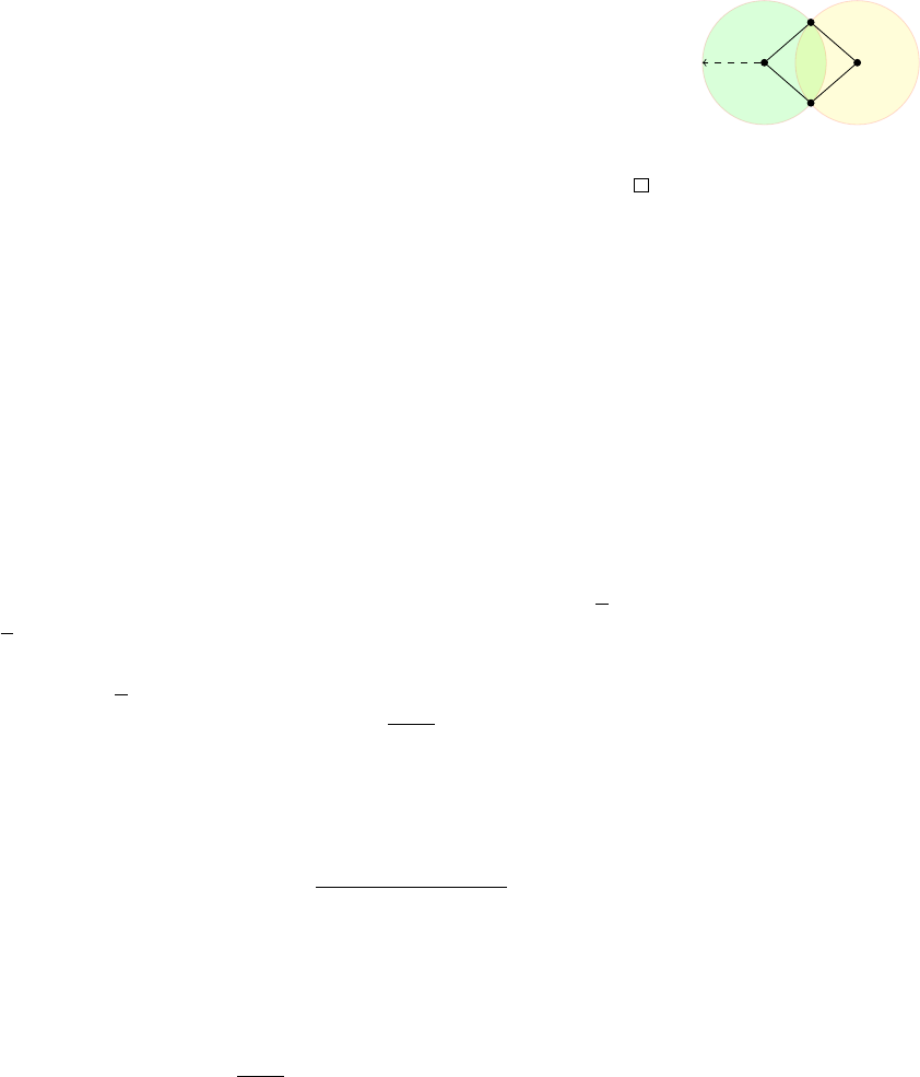
We are now ready to prove Schur’s theorem by setting up a graph
whose triangles correspond to solutions to x + y = z, thereby allow-
ing us to “transfer” the above result to the integers.
i j
k
φ(j −i) φ( k − j)
φ(k −i)
Proof of Schur’s theorem (Theorem 1.2). Let φ : [N] → [r] be a coloring.
Color the edges of a complete graph with vertices {1, . . . , N + 1} by
giving the edge {i, j} with i < j the color φ(j − i). By Theorem 1.4,
if N is large enough, then there is a monochromatic triangle, say on
vertices i < j < k. So φ (j − i) = φ(k − j) = φ(k − i). Take x = j − i,
y = k − j, and z = k −i. Then φ(x) = φ(y) = φ(z) and x + y = z, as
desired.
Notice how we solved a number theory problem by moving over
to a graph theoretic setup. The Ramsey theorem argument in Theo-
rem 1.4 is difficult to do directly inside the integers. Thus we gained
greater flexibility by considering graphs. Later on we will see other
more sophisticated examples of this idea, where taking a number
theoretic problem to the land of graph theory gives us a new perspec-
tive.
1.2 Highlights from additive combinatorics
Schur’s theorem above is one of the earliest examples of an area now
known as additive combinatorics, which is a term coined by Terry Green (2009)
Tao in the early 2000’s to describe a rapidly growing body of math-
ematics motivated by simple-to-state questions about addition and
multiplication of integers. The problems and methods in additive
combinatorics are deep and far-reaching, connecting many different
areas of mathematics such as graph theory, harmonic analysis, er-
godic theory, discrete geometry, and model theory. The rest of this
section highlights some important developments in additive combi-
natorics in the past century.
In the 1920’s, van der Waerden proved the following result about
monochromatic arithmetic progressions in the integers.
Theorem 1.5 (van der Waerden’s theorem). If the integers are colored B. L. van der Waerden, Beweis einer
Baudetschen Vermutung. Nieuw
Arch. Wisk. 15, 212–216, 1927.
with finitely many colors, then one of the color classes must contain arbi-
trarily long arithmetic progressions.
Remark 1.6. Having arbitrarily long arithmetic progressions is very
different from having infinitely long arithmetic progressions. As an
exercise, show that one can color the integers using just two colors so

16 highlights from additive combinatorics
that there are no infinitely long monochromatic arithmetic progres-
sions.
In the 1930’s, Erd˝os and Turán conjectured a stronger statement, Erd˝os and Turán (1936)
that any subset of the integers with positive density contains arbitrar-
ily long arithmetic progressions. To be precise, we say that A ⊆ Z
has positive upper density if
lim sup
N→∞
|A ∩{−N, . . . , N}|
2N + 1
> 0.
(There are several variations of this definition—the exact formulation
is not crucial.)
endre szemerédi (1940– ) received
the prestigious Abel Prize in 2012
“for his fundamental contributions to
discrete mathematics and theoretical
computer science, and in recognition
of the profound and lasting impact of
these contributions on additive number
theory and ergodic theory.”
In the 1950’s, Roth proved the conjecture for 3-term arithmetic
progression using Fourier analytic methods. In the 1970’s, Szemerédi
fully settled the conjecture using combinatorial techniques. These are
landmark theorems in the field. Much of what we will discuss are
motivated by these results and the developments around them.
Theorem 1.7 (Roth’s theorem). Every subset of the integers with positive
Roth (1953)
upper density contains a 3-term arithmetic progression.
Theorem 1.8 (Szemerédi’s theorem). Every subset of the integers with Szemerédi (1975)
positive upper density contains arbitrarily long arithmetic progressions.
Szemerédi’s proof was a combinatorial
tour de force. This figures is taken
from the introduction of his paper
showing the logical dependencies of his
argument.
Szemerédi’s theorem is deep and intricate. This important work
led to many subsequent developments in additive combinatorics.
Several different proofs of Szemerédi’s theorem have since been
discovered, and some of them have blossomed into rich areas of
mathematical research. Here are some the most influential modern
proofs of Szemerédi’s theorem (in historical order):
• The ergodic theoretic approach (Furstenberg)
Furstenberg (1977)
• Higher-order Fourier analysis (Gowers)
Gowers (2001)
• Hypergraph regularity lemma (Rödl et al./Gowers)
Rödl et al. (2005)
Gowers (2007)
Another modern proof of Szemerédi’s theorem results from the
density Hales–Jewett theorem, which was originally proved by Fursten-
berg and Katznelson using ergodic theory, and subsequently a new Furstenberg and Katznelson (1991)
Polymath (2012)
All subsequent Polymath Project papers
are written under the pseudonym
D. H. J. Polymath, whose initials stand
for “density Hales–Jewett.”
combinatorial proof was found in the first successful Polymath
Project, an online collaborative project initiated by Gowers.
The relationships between these disparate approaches are not yet
completely understood, and there are many open problems, espe-
cially regarding quantitative bounds. A unifying theme underlying
all known approaches to Szemerédi’s theorem is the dichotomy be- Tao (2007)
tween structure and pseudorandomness. We will later see different

introduction 17
facets of this dichotomy both in the context of graph theory as well as
in number theory.
Here are a few other important subsequent developments to Sze-
merédi’s theorem.
Instead of working over subsets of integers, let us consider subsets
of a higher dimensional lattice Z
d
. We say that A ⊂ Z
d
has positive
upper density if
lim sup
N→∞
|A ∩[−N, N]
d
|
(2N + 1)
d
> 0
(as before, other similar definitions are possible). We say that A con-
tains arbitrary constellations if for every finite set F ⊂ Z
d
, there is
some a ∈ Z
d
and t ∈ Z
>0
such that a + t · F = {a + tx : x ∈ F} is
contained in A. In other words, A contains every finite pattern, each
consisting of some finite subset of the integer grid allowing dilation
and translation. The following multidimensional generalization of
Szemerédi’s theorem was proved by Furstenberg and Katznelson ini-
tially using ergodic theory, though a combinatorial proof was later
discovered as a consequence of the hypergraph regularity method
mentioned earlier.
Theorem 1.9 (Multidimensional Szemerédi theorem). Every subset of Furstenberg and Katznelson (1978)
Z
d
of positive upper density contains arbitrary constellations.
For example, the theorem implies that every subset of Z
d
of pos-
itive upper density contains a 10 × 10 set of points that form an
axis-aligned square grid.
There is also a polynomial extension of Szemerédi’s theorem. Let
us first state a special case, originally conjectured by Lovász and
proved independently by Furstenberg and Sárk˝ozy.
Theorem 1.10. Any subset of the integers with positive upper density Furstenberg (1977)
Sárközy (1978)
contains two numbers differing by a square.
In other words, the set always contains {x, x + y
2
} for some x ∈ Z
and y ∈ Z
>0
. What about other polynomial patterns? The following
polynomial generalization was proved by Bergelson and Leibman.
Theorem 1.11 (Polynomial Szemerédi theorem). Suppose A ⊂ Z Bergelson and Leibman (1996)
has positive upper density. If P
1
, . . . , P
k
∈ Z[X] are polynomials with
P
1
(0) = ··· = P
k
(0) = 0, then there exist x ∈ Z and y ∈ Z
>0
such that
x + P
1
(y), . . . , x + P
k
(y) ∈ A.
We leave it as an exercise to formulate a common extension of the
above two theorems (i.e., a multidimensional polynomial Szemerédi
theorem). Such a theorem was also proved by Bergelson and Leib-
man.
18 what’s next?
We will not cover the proof of Theorems 1.9 and 1.11. In fact,
currently the only known general proof of the polynomial Szemerédi
theorem uses ergodic theory, though for special cases there are some
recent exciting developments. Peluse (2019+)
Building on Szemerédi’s theorem as well as other important de-
velopments in number theory, Green and Tao proved their famous
theorem that settled an old folklore conjecture about prime numbers.
Their theorem is considered one of the most celebrated mathematical
results this century.
Theorem 1.12 (Green–Tao theorem). The primes contain arbitrarily long Green and Tao (2008)
arithmetic progressions.
We will discuss many central ideas behind the proof of the Green–
Tao theorem. See the reference on the right for a modern exposition Conlon, Fox, and Zhao (2014)
of the Green–Tao theorem emphasizing the graph theoretic perspec-
tive, and incorporating some simplifications of the proof that have
been found since the original work.
1.3 What’s next?
One of our goals is to understand two different proofs of Roth’s
theorem, which can be rephrased as:
Theorem 1.13 (Roth’s theorem). Every subset of [N] that does not con-
tain 3-term arithmetic progressions has size o(N).
Roth originally proved his result using Fourier analytic techniques,
which we will see in the second half of this book. In the 1970’s, lead-
ing up to Szemerédi’s proof of his landmark result, Szemerédi de- Szemerédi (1978)
veloped an important tool known as the graph regularity lemma.
Ruzsa and Szemerédi used the graph regularity lemma to give a new Ruzsa and Szemerédi (1978)
graph theoretic proof of Roth’s theorem. One of our first goals is to
understand this graph theoretic proof.
As in the proof of Schur’s theorem, we will formulate a graph
theoretic problem whose solution implies Roth’s theorem. This topic
fits nicely in an area of combinatorics called extremal graph theory. A
starting point (historically and also pedagogically) in extremal graph
theory is the following question:
Question 1.14. What is the maximum number of edges in a triangle-
free graph on n vertices?
This question is relatively easy, and it was answered by Mantel in
the early 1900’s (and subsequently rediscovered and generalized by
Turán). It will be the first result that we shall prove next. However,
even though it sounds similar to Roth’s theorem, it cannot be used to
introduction 19
deduce Roth’s theorem. Later on, we will construct a graph that cor-
responds to Roth’s theorem, and it turns out that the right question
to ask is:
Question 1.15. What is the maximum number of edges in an n-vertex
graph where every edge is contained in a unique triangle?
This innocent looking question turns out to be incredible myste-
rious. We are still far from knowing the truth. We will later prove,
using Szemerédi’s regularity lemma, that any such graph must have
o(n
2
) edges, and we will then deduce Roth’s theorem from this graph
theoretic claim.
Part I
Graph theory

2
Forbidding subgraphs
9/11: Anlong Chua and Chris Xu
2.1 Mantel’s theorem: forbidding a triangle
We begin our discussion of extremal graph theory with the following
basic question.
Question 2.1. What is the maximum number of edges in an n-vertex
graph that does not contain a triangle?
Bipartite graphs are always triangle-free. A complete bipartite
graph, where the vertex set is split equally into two parts (or differing
by one vertex, in case n is odd), has
n
2
/4
edges. Mantel’s theorem
states that we cannot obtain a better bound:
Theorem 2.2 (Mantel). Every triangle-free graph on n vertices has at W. Mantel, "Problem 28 (Solution by H.
Gouwentak, W. Mantel, J. Teixeira de
Mattes, F. Schuh and W. A. Wythoff).
Wiskundige Opgaven 10, 60 —61, 1907.
most bn
2
/4c edges.
We will give two proofs of Theorem 2.2.
Proof 1. Let G = (V, E) a triangle-free graph with n vertices and m
edges. Observe that for distinct x, y ∈ V such that xy ∈ E, x and y
must not share neighbors by triangle-freeness.
x
y
N(x)
N(y)
Adjacent vertices have disjoint neigh-
borhoods in a triangle-free graph.
Therefore, d(x) + d(y) ≤ n, which implies that
∑
x∈V
d(x)
2
=
∑
xy∈E
(
d(x) + d(y)
)
≤ mn.
On the other hand, by the handshake lemma,
∑
x∈V
d(x) = 2m. Now
by the Cauchy–Schwarz inequality and the equation above,
4m
2
=
∑
x∈V
d(x)
!
2
≤ n
∑
x∈V
d(x)
2
!
≤ mn
2
;
hence m ≤ n
2
/4. Since m is an integer, this gives m ≤ bn
2
/4c.
Proof 2. Let G = (V, E) be as before. Since G is triangle-free, the
neighborhood N(x) of every vertex x ∈ V is an independent set.
x
y
z
An edge within N(x) creates a triangle

24 turán’s theorem: forbidding a clique
Let A ⊆ V be a maximum independent set. Then d(x) ≤ |A| for
all x ∈ V. Let B = V \ A. Since A contains no edges, every edge of G
intersects B. Therefore,
e(G) ≤
∑
x∈B
d(x) ≤ |A||B|
≤
AM-GM
$
|A| + |B|
2
2
%
=
n
2
4
.
Remark 2.3. For equality to occur in Mantel’s theorem, in the above
proof, we must have
• e(G) =
∑
x∈B
d(x), which implies that no edges are strictly in B.
•
∑
x∈B
d(x) = |A||B|, which implies that every vertex in B is com-
plete in A.
• The equality case in AM-GM must hold (or almost hold, when n is
odd), hence
|
|A| − |B|
|
≤ 1.
Thus a triangle-free graph on n vertices has exactly
n
2
/4
edges if
and only if it is the complete bipartite graph K
b
n/2
c
,
d
n/2
e
.
2.2 Turán’s theorem: forbidding a clique
Motivated by Theorem 2.2, we turn to the following more general
question.
Question 2.4. What is the maximum number of edges in a K
r+1
-free
graph on n vertices?
Extending the bipartite construction earlier, we see that an r-partite
graph does not contain any copy of K
r+1
.
Definition 2.5. The Turán graph T
n,r
is defined to be the complete,
n-vertex, r-partite graph, with part sizes either
n
r
or
n
r
.
The Turán graph T
10,3
In this section, we prove that T
n,r
does, in fact, maximize the num-
ber of edges in a K
r
-free graph:
Theorem 2.6 (Turán). If G is an n-vertex K
r+1
-free graph, then e(G) ≤
P. Turán, On an extremal problem in
graph theory. Math. Fiz. Lapok 48, 436
—452, 1941.
e(T
n,r
).
When r = 2, this is simply Theorem 2.2.
We now give three proofs of Theorem 2.6. The first two are in the
same spirit as the proofs of Theorem 2.2.

forbidding subgraphs 25
Proof 1. Fix r. We proceed by induction on n. Observe that the state-
ment is trivial if n ≤ r, as K
n
is K
r+1
-free. Now, assume that n > r
and that Turán’s theorem holds for all graphs on fewer than n ver-
tices. Let G be an n-vertex, K
r+1
-free graph with the maximum pos-
sible number of edges. Note that G must contain K
r
as a subgraph,
or else we could add an edge in G and still be K
r+1
-free. Let A be the
vertex set of an r-clique in G, and let B := V\A. Since G is K
r+1
-free,
every v ∈ B has at most r −1 neighbors in A. Therefore
e(G) ≤
r
2
+ ( r −1)|B| + e(B)
≤
r
2
+ ( r −1)(n −r) + e(T
n−r,r
)
= e(T
n,r
).
The first inequality follows from counting the edges in A, B, and
everything in between. The second inequality follows from the in-
ductive hypothesis. The last equality follows by noting removing
one vertex from each of the r parts in T
n,r
would remove a total of
(
r
2
)
+ ( r −1)(n −r) edges.
Proof 2 (Zykov symmetrization). As before, let G be an n-vertex, K
r+1
-
free graph with the maximum possible number of edges.
We claim that the non-edges of G form an equivalence relation;
that is, if xy, yz /∈ E, then xz /∈ E. Symmetry and reflexivity are easy
to check. To check transitivity, Assume for purpose of contradiction
that there exists x, y, z ∈ V for which xy, yz /∈ E but xz ∈ E.
If d(y) < d(x), we may replace y with a “clone” of x. That is, we
delete y and add a new vertex x
0
whose neighbors are precisely the
as the neighbors of x (and no edge between x and x
0
). (See figure on
the right.)
x
x
0
x and its clone x
0
Then, the resulting graph G
0
is also K
r+1
-free since x was not in
any K
r+1
. On the other hand, G
0
has more edges than G, contradict-
ing maximality.
Therefore we have that d(y) ≥ d(x) for all xy /∈ E. Similarly,
d(y) ≥ d(z). Now, replace both x and z by “clones” of y. The new
graph G
0
is K
r+1
-free since y was not in any K
r+1
, and
e(G
0
) = e(G) − ( d(x) + d(z) −1) + 2d(y) > e(G),
contradicting maximality of e(G). Therefore such a triple (x, y, z)
cannot exist in G, and transitivity holds.
The equivalence relation shows that the complement of G is a
union of cliques. Therefore G is a complete multipartite graph with
at most r parts. One checks that increasing the number of parts in-
creases the number of edges in G. Similarly, one checks that if the

26 hypergraph turán problem
number of vertices in two parts differ by more than 1, moving one
vertex from the larger part to the smaller part increases the number
of edges in G. It follows that the graph that achieves the maximum
number of edges is T
n,r
.
Our third and final proof uses a technique called the probabilistic
method. In this method, one introduces randomness to a determinis-
tic problem in a clever way to obtain deterministic results.
Proof 3. Let G = (V, E) be an n-vertex, K
r+1
-free graph. Consider a
uniform random ordering σ of the vertices. Let
X = {v ∈ V : v is adjacent to all earlier vertices in σ}.
Observe that the set of vertices in X form a clique. Since the permuta-
tion was chosen uniformly at random, we have
P(v ∈ X) = P(v appears before all non-neighbors) =
1
n − d(v)
.
Therefore,
r ≥ E|X| =
∑
v∈V
P(v ∈ X) =
∑
v∈V
1
n − d(v)
convexity
≥
n
n −2m/n
.
Rearranging gives m ≤
1 −
1
r
n
2
2
(a bound that is already good for
most purposes). Note that if n is divisible by r, then the bound imme-
diately gives a proof of Turán’s theorem. When n is not divisible by
r, one needs to a bit more work and use convexity to argue that the
d(v) should be as close as possible. We omit the details.
2.3 Hypergraph Turán problem
The short proofs given in the previous sections make problems in
extremal graph theory seem deceptively simple. In reality, many
generalizations of what we just discussed remain wide open.
Here we discuss one notorous open problem that is a hypergraph
generalization of Mantel/Turán.
An r-uniform hypergraph consists of a vertex set V and an edge
set, where every edge is now an r-element subset of V. Graphs corre-
spond to r = 2.
Question 2.7. What is the maximum number of triples in an n vertex
3-uniform hypergraph without a tetrahedron?
Turán proposed the following construction, which is conjectured to
be optimal.

forbidding subgraphs 27
Example 2.8 (Turán). Let V be a set of n vertices. Partition V into
3 (roughly) equal sets V
1
, V
2
, V
3
. Add a triple {x, y, z} to e(G) if it
satisfies one of the four following conditions:
• x, y, z are in different partitions
• x, y ∈ V
1
and z ∈ V
2
• x, y ∈ V
2
and z ∈ V
3
• x, y ∈ V
3
and z ∈ V
1
where we consider x, y, z up to permutation (See Example 2.8). One
checks that the 3-uniform hypergraph constructed is tetrahedron-free,
and that it has edge density 5/9.
Turán’s construction of a tetrahedron-
free 3-uniform hypergraph
On the other hand, the best known upper bound is approximately
0.562 , obtained recently using the technique of flag algebras.
Keevash (2011)
Baber and Talbot (2011)
Razborov (2010)
2.4 Erd˝os–Stone–Simonovits theorem (statement): forbidding a
general subgraph
One might also wonder what happens if K
r+1
in Theorem 2.6 were
replaced with an arbitrary graph H:
Question 2.9. Fix some graph H. If G is an n vertex graph in which
H does not appear as a subgraph, what is the maximum possible
number of edges in G?
Notice that we only require H to be a
subgraph, not necessarily an induced
subgraph. An induced subgraph H
0
of G must contain all edges present
between the vertices of H
0
, while there
is no such restriction for arbitrary
subgraphs.
Definition 2.10. For a graph H and n ∈ N, define ex(n, H) to be the
maximum number of edges in an n-vertex H-free graph.
For example, Theorem 2.6 tells us that for any given r,
ex(n, K
r+1
) = e(T
n,r
) =
1 −
1
r
+ o(1)
n
2
where o(1) represents some quantity that goes to zero as n → ∞.
At a first glance, one might not expect a clean answer to Ques-
tion 2.9. Indeed, the solution would seem to depend on various char-
acteristics of H (for example, its diameter or maximum degree). Sur-
prisingly, it turns out that a single parameter, the chromatic number
of H, governs the growth of ex(n, H).
Definition 2.11. The chromatic number of a graph G, denoted χ(G),
is the minimal number of colors needed to color the vertices of G
such that no two adjacent vertices have the same color.
Example 2.12. χ( K
r+1
) = r + 1 and χ(T
n,r
) = r.

28 k
˝
ovári–sós–turán theorem: forbidding a complete bipartite graph
Observe that if H ⊆ G, then χ(H) ≤ χ(G). Indeed, any proper
coloring of G restricts to a proper coloring of H. From this, we gather
that if χ(H) = r + 1, then T
n,r
is H-free. Therefore,
ex(n, H) ≥ e(T
n,r
) =
1 −
1
r
+ o(1)
n
2
.
Is this the best we can do? The answer turns out to be affirmative.
Theorem 2.13 (Erd˝os–Stone–Simonovits). For all graphs H, we have Erd˝os and Stone (1946)
Erd˝os and Simonovits (1966)
lim
n→∞
ex(n, H)
(
n
2
)
= 1 −
1
χ(H) −1
.
We’ll skip the proof for now.
Remark 2.14. Later in the book we will show how to deduce Theo-
rem 2.13 from Theorem 2.6 using the Szemerédi regularity lemma.
Example 2.15. When H = K
3
, Theorem 2.13 tells us that
lim
n→∞
ex(n, H)
(
n
2
)
=
1
2
,
in agreement with Theorem 2.6.
When H = K
4
, we get
lim
n→∞
ex(n, H)
(
n
2
)
=
2
3
,
also in agreement with Theorem 2.6.
When H is the Peterson graph, Theorem 2.13 tells us that
lim
n→∞
ex(n, H)
(
n
2
)
=
1
2
,
which is the same answer as for H = K
3
! This is surprising since the
Peterson graph seems much more complicated than the triangle.
1
2
3
1
3
2
2
3
2
1
The Peterson graph with a proper
3-coloring.
2.5 K˝ovári–Sós–Turán theorem: forbidding a complete bipartite
graph
9/16: Jiyang Gao and Yinzhan Xu
The Erd˝os–Stone–Simonovits Theorem (Theorem 2.13) gives a first-
order approximation of ex(n, H) when χ(H) > 2. Unfortunately,
Theorem 2.13 does not tell us the whole story. When χ(H) = 2, i.e.
H is bipartite, the theorem implies that ex(n, H) = o(n
2
), which com-
pels us to ask if we may obtain more precise bounds. For example, if
we write ex(n, H) as a function of n, what its growth with respect to
n? This is an open problem for most bipartite graphs (for example,
K
4,4
) and the focus of the remainder of the chapter.
Let K
s,t
be the complete bipartite graph where the two parts of the
bipartite graph have s and t vertices respectively. In this section, we
consider ex(n, K
s,t
), and seek to answer the following main question:
An example of a complete bipartite
graph K
3,5
.

forbidding subgraphs 29
Question 2.16 (Zarankiewicz problem). For some r, s ≥ 1, what is
the maximum number of edges in an n-vertex graph which does not
contain K
s,t
as a subgraph.
Every bipartite graph H is a subgraph of some complete bipartite
graph K
s,t
. If H ⊆ K
s,t
, then ex(n, H) ≤ ex(n, K
s,t
). Therefore, by
understanding the upper bound on the extremal number of complete
bipartite graphs, we obtain an upper bound on the extremal number
of general bipartite graphs as well. Later, we will give improved
bounds for several specific biparite graphs.
K˝ovári, Sós and Turán gave an upper bound on K
s,t
:
Theorem 2.17 (K˝ovári–Sós–Turán). For every integers 1 ≤ s ≤ t, there K˝ovári, Sós, and Turán (1954)
exists some constant C, such that
ex(n, K
s,t
) ≤ Cn
2−
1
s
.
There is an easy way to remember
the name of this theorem: “KST”, the
initials of the authors, is also the letters
for the complete bipartite graph K
s,t
.
Proof. Let G be a K
s,t
-free n-vertex graph with m edges.
First, we repeatedly remove all vertices v ∈ V(G) where d(v) <
s −1. Since we only remove at most (s −2)n edges this way, it suffices
to prove the theorem assuming that all vertices have degree at least
s −1.
We denote the number of copies of K
s,1
in G as #K
s,1
. The proof
establishes an upper bound and a lower bound on #K
s,1
, and then
gets a bound on m by combining the upper bound and the lower
bound.
Since K
s,1
is a complete bipartite graph, we can call the side with s
vertices the ‘left side‘, and the side with 1 vertices the ‘right side‘.
On the one hand, we can count #K
s,1
by enumerating the ‘left side‘.
For any subset of s vertices, the number of K
s,1
where these s vertices
form the ‘left side‘ is exactly the number of common neighbors of
these s vertices. Since G is K
s,t
-free, the number of common neigh-
bors of any subset of s vertices is at most t − 1. Thus, we establish
that #K
s,1
≤
(
n
s
)
(t −1).
On the other hand, for each vertex v ∈ V(G), the number of copies
of K
s,1
where v is the ‘right side‘ is exactly
(
d(v)
s
)
. Therefore, Here we regard
(
x
s
)
as a degree s poly-
nomial in x, so it makes sense for x to
be non-integers. The function
(
x
s
)
is
convex when x ≥ s − 1.
#K
s,1
=
∑
v∈V(G)
d(v)
s
≥ n
1
n
∑
v∈V(G)
d(v)
s
= n
2m/n
s
,
where the inequality step uses the convextiy of x 7→
(
x
s
)
.
Combining the upper bound and lower bound of #K
s,1
, we obtain
that n
(
2m/n
s
)
≤
(
n
s
)
(t − 1). For constant s, we can use
(
x
s
)
= (1 +
o(1))
n
s
s!
to get n
2m
n
s
≤ (1 + o(1))n
s
(t − 1). The above inequality
simplifies to
m ≤
1
2
+ o(1)
(t −1)
1/s
n
2−
1
s
.

30 k
˝
ovári–sós–turán theorem: forbidding a complete bipartite graph
Let us discuss a geometric application of Theorem 2.17.
Question 2.18 (Unit distance problem). What is the maximum num- Erd˝os (1946)
ber of unit distances formed by n points in R
2
?
For small values of n, we precisely know the answer to the unit
distance problem. The best configurations are listed in Figure 2.1.
n = 3 n = 4 n = 5
n = 6 n = 7
Figure 2.1: The configurations of points
for small values of n with maximum
number of unit distances. The edges
between vertices mean that the distance
is 1. These constructions are unique up
to isomorphism except when n = 6.
It is possible to generalize some of these constructions to arbitrary
n.
• A line graph has (n −1) unit distances.
···
• A chain of triangles has (2n −3) unit distances for n ≥ 3.
···
P
P
0
1
• There is also a recursive construction. Given a configuration P
with n/2 points that have f (n/2) unit distances, we can copy P
and translate it by an arbitrary unit vector to get P
0
. The configu-
ration P ∪ P
0
have at least 2 f (n/2) + n/2 unit distances. We can
solve the recursion to get f (n) = Ω(n log n).
The current best lower bound on the maximum number of unit dis-
tances is given by Erd˝os.
Proposition 2.19. There exists a set of n points in R
2
that have at least Erd˝os (1946)
n
1+c/ log log n
unit distances for some constant c.
Figure 2.2: An example grid graph
where n = 25 and r = 10.
Proof sketch. Consider a square grid with b
√
nc ×b
√
nc vertices. We
can scale the graph arbitrarily so that
√
r becomes the unit distance
for some integer r. We can pick r so that r can be represented as a
sum of two squares in many different ways. One candidate of such
r is a product of many primes that are congruent to 1 module 4. We
can use some number-theoretical theorems to analyze the best r, and
get the n
1+c/ log log n
bound.
Theorem 2.17 can be used to prove an upper bound on the number
of unit distances.
Theorem 2.20. Every set of n points in R
2
has at most O(n
3/2
) unit
distances.
Proof. Given any set of points S ⊂ R
2
, we can create the unit distance
graph G as follows:
• The vertex set of G is S,
• For any point p, q where d(p, q) = 1, we add an edge between p
and q.
forbidding subgraphs 31
p q
r = 1
Figure 2.3: Two vertices p, q can have at
most two common neighbors in the unit
distance graph.
The graph G is K
2,3
-free since for every pair of points p, q, there are at
most 2 points that have unit distances to both of them. By applying
Theorem 2.17, we obtain that e(G) = O(n
3/2
).
Remark 2.21. The best known upper bound on the number of unit Spencer, Szemerédi and Trotter (1984)
distances is O(n
4/3
). The proof is a nice application of the crossing
number inequality which will be introduced later in this book.
Here is another problem that is strongly related to the unit dis-
tance problem:
Question 2.22 (Distinct distance problem). What is the minimum
number of distinct distances formed by n points in R
2
?
Example 2.23. Consider n points on the x-axis where the i-th point
has coordinate (i, 0). The number of distinct distances for these
points is n −1.
The current best construction for minimum number of distinct
distances is also the grid graph. Consider a square grid with b
√
nc ×
b
√
nc vertices. Possible distances between two vertices are numbers
that can be expressed as a sum of the squares of two numbers that
are at most b
√
nc. Using number-theoretical methods, we can obtain
that the number of such distances: Θ(n/
p
log n).
The maximum number of unit distances is also the maximum
number that each distance can occur. Therefore, we have the follow-
ing relationship between distinct distances and unit distances:
#distinct distances ≥
(
n
2
)
max #unit distances
.
If we apply Theorem 2.20 to the above inequality, we immediately get
an Ω (n
0.5
) lower bound for the number of distinct distances. Many
mathematicians successively improved the exponent in this lower
bound over the span of seven decades. Recently, Guth and Katz gave
the following celebrated theorem, which almost matches the upper
bound (only off by an O(
p
log n)) factor).
Theorem 2.24 (Guth–Katz). Every set of n points in R
2
has at least Guth and Katz (2015)
cn/ log n distinct distances for some constant c.
The proof of Theorem 2.24 is quite sophisticated: it uses tools
ranging from polynomial method to algebraic geometry. We won’t
cover it in this book.
2.6 Lower bounds: randomized constructions
It is conjectured that the bound proven in Theorem 2.17 is tight. In
other words, ex(n, K
s,t
) = Θ(n
2−1/s
). Although this still remains

32 lower bounds: randomized constructions
open for arbitrary K
s,t
, it is already proven for a few small cases,
and in cases where t is way larger than s. In this and the next two
sections, we will show techniques for constructing H-free graphs.
Here are the three main types of constructions that we will cover:
• Randomized construction. This method is powerful and general,
but introducing randomness means that the constructions are
usually not tight.
• Algebraic construction. This method uses tools in number theory
or algebra to assist construction. It gives tighter results, but they
are usually ‘magical’, and only works in a small set of cases.
• Randomized algebraic construction. This method is the hybrid of
the two methods above and combines the advantages of both.
This section will focus on randomized constructions. We start with a
general lower bound for extremal numbers.
Theorem 2.25. For any graph H with at least 2 edges, there exists a con-
stant c > 0, such that for any n ∈ N, there exists an H-free graph on n
vertices with at least cn
2−
v(H)−2
e(H)−1
edges. In other words,
ex(n, H) ≥ cn
2−
v(H)−2
e(H)−1
.
Proof. The idea is to use the alteration method: we can construct a
graph that has few copies of H in it, and delete one edge from each
copy to eliminate the occurrences of H. The random graph G(n, p) is called
the Erd˝os–Rényi random graph, which
appears in many randomized construc-
tions.
Consider G = G(n, p) as a random graph with n vertices where
each edge appears with probability p (p to be determined). Let #H be
the number of copies of H in G. Then,
E[#H] =
n(n −1) ···(n −v(H) + 1)
|Aut(H)|
p
e(H)
≤ p
e(H)
n
v(H)
,
where Aut(H) is the automorphism group of graph H, and
E[e(G)] = p
n
2
.
Let p =
1
2
n
−
v(H)−2
e(H)−1
, chosen so that
E[#H] ≤
1
2
E[e(G)],
which further implies
E[e(G) −#H] ≥
1
2
p
n
2
≥
1
16
n
2−
v(H)−2
e(H)−1
.
Thus, there exists a graph G, such that the value of (e(G) − #H) is
at least the expectation. Remove one edge from each copy of H in G,
and we get an H-free graph with enough edges.

forbidding subgraphs 33
Remark 2.26. For example, if H is the following graph
then applying Theorem 2.25 directly gives
ex(n, H) & n
11/7
.
However, if we forbid H’s subgraph K
4
instead (forbidding a sub-
graph will automatically forbid the original graph), Theorem 2.25
actually gives us a better bound:
ex(n, H) ≥ ex(n, K
4
) & n
8/5
.
For a general H, we apply Theorem 2.25 to the subgraph of H with
the maximum (e − 1)/(v − 2) value. For this purpose, define the
2-density of H as
m
2
(H) := max
H
0
⊆H
v(H
0
)≥3
e(H
0
) −1
v(H
0
) −2
.
We have the following corollary.
Corollary 2.27. For any graph H with at least two edges, there exists
constant c = c
H
> 0 such that
ex(n, H) ≥ cn
2−1/m
2
(H)
.
Example 2.28. We present some specific examples of Theorem 2.25.
This lower bound, combined with the upper bound from the K˝ovári–
Sós–Turán theorem (Theorem 2.17), gives that for every 2 ≤ s ≤ t,
n
2−
s+t−2
st−1
. ex(n, K
s,t
) . n
2−1/s
.
When t is large compared to s, the exponents in the two bounds
above are close to each other (but never equal).
When t = s, the above bounds specialize to
n
2−
2
s+1
. n
2−
s+t−2
st−1
.. n
2−1/s
.
In particular, for s = 2, we obtain
n
4/3
. ex(n, K
2,2
) . n
3/2
.
It turns out what the upper bound is close to tight, as we show next a
different, algebraic, construction of a K
2,2
-free graph.

34 lower bounds: algebraic constructions
2.7 Lower bounds: algebraic constructions
In this section, we use algebraic constructions to find K
s,t
-free graphs,
for various values of (s, t), that match the upper bound in the K˝ovári–
Sós–Turán theorem (Theorem 2.17) up to a constant factor.
The simplest example of such an algebraic construction is the
following construction of K
2,2
-free graphs with many edges.
Theorem 2.29 (Erd˝os–Rényi–Sós). Erd˝os, Rényi and Sós (1966)
ex(n, K
2,2
) ≥
1
2
−o(1)
n
3/2
.
Proof. Suppose n = p
2
−1 where p is a prime. Consider the following
graph G (called polarity graph): Why is it called a polarity graph? It
may be helpful to first think about
the partite version of the construction,
where one vertex set is the set of points
of of a (projective) plane over F
p
, and
the other vertex set is the set of lines in
the same plane, and one has an edge
between point p and line ` if p ∈ `.
This graph is C
4
-free since no two lines
intersect in two distinct points.
The construction in the proof of
Theorem 2.29 has one vertex set that
identifies points with lines. This duality
pairing between points and lines
is known in projective geometry a
polarity.
• V(G) = F
2
p
\{(0, 0)},
• E(G) = {(x, y) ∼ (a, b)|ax + by = 1 in F
p
}.
For any two distinct vertices (a, b) 6= (a
0
, b
0
) ∈ V(G), there is at
most one solution (common neighbour) (x, y) ∈ V(G) satisfying both
ax + by = 1 and a
0
x + b
0
y = 1. Therefore, G is K
2,2
-free.
Most vertices have degree p because
the equation ax + by = 1 has exactly p
solutions (x, y). Sometimes we have to
subtract 1 because one of the solutions
might be (a, b) itself, which forms a
self-loop.
Moreover, every vertex has degree p or p −1, so the total number
of edges
e(G) =
1
2
−o(1)
p
3
=
1
2
−o(1)
n
3/2
,
which concludes our proof.
If n does not have the form p
2
− 1 for some prime, then we let p
be the largest prime such that p
2
− 1 ≤ n. Then p = (1 − o(1)n
and constructing the same graph G
p
2
−1
with n − p
2
+ 1 isolated
Here we use that the smallest prime
greater than n has size n + o(n) . The
best result of this form says that there
exists a prime in the interval [n −
n
0.525
, n] for every sufficiently large n.
Baker, Harman and Pintz (2001)
vertices.
A natural question to ask here is whether the construction above
can be generalized. The next construction gives us a construction for
K
3,3
-free graphs.
Theorem 2.30 (Brown). Brown (1966)
It is known that the constant 1/2 in
Theorem 2.30 is the best constant
possible.
ex(n, K
3,3
) ≥
1
2
−o(1)
n
5/3
Proof sketch. Let n = p
3
where p is a prime. Consider the following
graph G:
• V(G) = F
3
p
• E(G) = {(x, y, z) ∼ (a, b, c)|(a − x)
2
+ (b − y)
2
+ (c − z)
2
=
u in F
p
}, where u is some carefully-chosen fixed nonzero element
in F
p

forbidding subgraphs 35
One needs to check that it is possible to choose u so that the above
graph is K
3,3
. We omit the proof but give some intuition. Had we
used points in R
3
instead of F
3
p
, the K
3,3
-freeness is equivalent to the
statement that three unit spheres have at most two common points.
This statement about unit spheres in R
3
, and it can be proved rigor-
ously by some algebraic manipulation. One would carry out a similar
algebraic manipulation over F
p
to verify that the graph above is K
3,3
-
free.
Moreover, each vertex has degree around p
2
since the distribution
of (a −x)
2
+ (b −y)
2
+ (c −z)
2
is almost uniform across F
p
as (x, y, z)
varies randomly over F
3
p
, and so we expect roughly a 1/p fraction of
(x, y, z) to have (a −x)
2
+ (b −y)
2
+ (c −z)
2
= u. Again we omit the
details.
Although the case of K
2,2
and K
3,3
are fully solved, the correspond-
ing problem for K
4,4
is a central open problem in extremal graph
theory.
Open problem 2.31. What is the order of growth of ex(n, K
4,4
)? Is it
Θ(n
7/4
), matching the upper bound in Theorem 2.17?
9/18: Michael Ma
We have obtained the K˝ovári–Sós–Turán bound up to a constant
factor for K
2,2
and K
3,3
. Now we present a construction that matches
the K˝ovári–Sós–Turán bound for K
s,t
whenever t is sufficiently large
compared to s.
Theorem 2.32 (Alon, Kollár, Rónyai, Szabó). If t ≥ (s −1)! + 1 then Kollár, Rónyai, and Szabó (1996)
Alon, Rónyai, and Szabó (1999)
ex(n, K
s,t
) = Θ(n
2−
1
s
).
We begin by proving a weaker version for t ≥ s! + 1. This will be
similar in spirit and later we will make an adjustment to achieve the
desired bound. Take a prime p and n = p
s
with s ≥ 2. Consider the Notice that we said the image of N
lies in F
p
rather than F
p
s
. We can
easily check this is indeed the case as
N(x)
p
= N(x) .
norm map N : F
p
s
→ F
p
defined by
N(x) = x ·x
p
· x
p
2
···x
p
s−1
= x
p
s
−1
p−1
.
Define the graph NormGraph
p,s
= (V, E) with
V = F
p
s
and E = {{a, b}|a 6= b, N(a + b) = 1}.
Proposition 2.33. In NormGraph
p,s
defined as above, letting n = p
s
be the
number of vertices,
|E| ≥
1
2
n
2−
1
s
.
Proof. Since F
×
p
s
is a cyclic group of order p
s
−1 we know that
|{x ∈ F
p
s
|N(x) = 1}| =
p
s
−1
p −1
.

36 lower bounds: algebraic constructions
Thus for every vertex x (the minus one accounts for vertices with
N(x + x) = 1)
deg(x) ≥
p
s
−1
p −1
−1 ≥ p
s−1
= n
1−
1
s
.
This gives us the desired lower bound on the number of edges.
Proposition 2.34. NormGraph
p,s
is K
s,s!+1
-free.
We wish to upper bound the number of common neighbors to a
set of s vertices. We quote without proof the following result, which
can be proved using algebraic geometry.
Theorem 2.35. Let F be any field and a
ij
, b
i
∈ F such that a
ij
6= a
i
0
j
for all Kollár, Rónyai, and Szabó (1996)
i 6= i
0
. Then the system of equations
(x
1
− a
11
)(x
2
− a
12
) ···(x
s
− a
1s
) = b
1
(x
1
− a
21
)(x
2
− a
22
) ···(x
s
− a
2s
) = b
2
.
.
.
(x
1
− a
s1
)(x
2
− a
s2
) ···(x
s
− a
ss
) = b
s
has at most s! solutions in F
s
.
Remark 2.36. Consider the special case when all the b
i
are 0. In this
case, since the a
ij
are distinct for a fixed j, we are picking an i
j
for
which x
j
= a
i
j
j
. Since all the i
j
are distinct, this is equivalent to
picking a permutation on [s]. Therefore there are exactly s! solutions.
We can now prove Proposition 2.34.
Proof of Proposition 2.34. Consider distinct y
1
, y
2
, . . . , y
s
∈ F
p
s
. We
wish to bound the number of common neighbors x. We can use the
fact that in a field with characteristic p we have (x + y)
p
= x
p
+ y
p
to
obtain
1 = N(x + y
i
) = (x + y
i
)(x + y
i
)
p
. . . (x + y
i
)
p
s−1
= (x + y
i
)(x
p
+ y
p
i
) . . . (x
p
s−1
+ y
p
s−1
i
)
for all 1 ≤ i ≤ s. By Theorem 2.35 these s equations have at most
s! solutions in x. Notice we do in fact satisfy the hypothesis since
y
p
i
= y
p
j
if and only if y
i
= y
j
in our field.
Now we introduce the adjustment to achieve the bound t ≥ (s −
1)! + 1 in Theorem 2.32. We define the graph ProjNormGraph
p,s
=
(V, E) with V = F
p
s−1
×F
×
p
for s ≥ 3. Here n = (p −1)p
s−1
. Define
the edge relation as (X, x) ∼ (Y, y) if and only if
N(X + Y) = xy.

forbidding subgraphs 37
Proposition 2.37. In ProjNormGraph
p,s
defined as above, letting n =
(p −1)p
s−1
denote the number of vertices,
|E| =
1
2
−o(1)
n
2−
1
s
.
Proof. It follows from that every vertex (X, x) has degree p
s−1
−1 =
(1 −o(1))n
1−1/s
since its neighbors are (Y, N(X + Y)/x) as Y ranges
over elements of F
p
s−1
over than −X.
Now that we know we have a sufficient amount of edges we just
need our graph to be K
s,(s−1)!+1
-free.
Proposition 2.38. ProjNormGraph
p,s
is K
s,(s−1)!+1
-free.
Proof. Once again we fix distinct (Y
i
, y
i
) ∈ V for 1 ≤ i ≤ s and we
wish to find all common neighbors (X, x). Then
N(X + Y
i
) = xy
i
.
Assume this system has at least one solution. Then if Y
i
= Y
j
with i 6=
j we must have that y
i
= y
j
. Therefore all the Y
i
are distinct. For each
i < s we can take N(X + Y
i
) = xy
i
and divide by N(X + Y
s
) = xy
s
to
obtain
N
X + Y
i
X + Y
s
=
y
i
y
s
.
Dividing both sides by N(Y
i
−Y
s
) we obtain
N
1
X + Y
s
+
1
Y
i
−Y
s
=
y
i
N(Y
i
−Y
s
)y
s
for all 1 ≤ i ≤ s − 1. Now applying Theorem 2.35 there are at most
(s − 1)! choices for X, which also determines x = N(X + Y
1
)/y
1
.
Thus there are at most (s −1)! common neighbors.
Now we are ready to prove Theorem 2.32.
Proof of Theorem 2.32. By Proposition 2.37 and Proposition 2.38 we
know that ProjNormGraph
p,s
is K
s,(s−1)!+1
-free and therefore K
s,t
-free
and has
1
2
−o(1)
n
2−
1
s
edges as desired.
2.8 Lower bounds: randomized algebraic constructions
So far we have seen both constructions using random graphs and
algebraic constructions. In this section we present an alternative
construction of K
s,t
-free graphs due to Bukh with Θ(n
2−
1
s
) edges pro- Bukh (2015)
vided t > t
0
(s) for some function t
0
. This is an algebraic construction
with some randomness added to it.

38 lower bounds: randomized algebraic constructions
First fix s ≥ 4 and take a prime power q. Let d = s
2
− s + 2 and
f ∈ F
q
[x
1
, x
2
, . . . , x
s
, y
1
, y
2
, . . . , y
s
] be a polynomial chosen uniformly
at random among all polynomials with degree at most d in each
of X = (x
1
, x
2
, . . . , x
s
) and Y = (y
1
, y
2
, . . . , y
s
). Take G bipartite
with vertex parts n = L = R = F
s
q
and define the edge relation as
(X, Y) ∈ L ×R when f (X, Y) = 0.
Lemma 2.39. For all u, v ∈ F
s
q
and f chosen randomly as above
P[ f (u, v) = 0] =
1
q
.
Proof. Notice that if g is a uniformly random constant in F
q
, then
f (u, v) and f (u, v) + g are identically distributed. Hence each of the q
possibilities are equally likely to the probability is 1/q.
Now the expected number of edges is the order we want as
E[e(G)] =
n
2
q
. All that we need is for the number of copies of K
s,t
to be relatively low. In order to do so, we must answer the follow-
ing question. For a set of vertices in L of size s, how many common
neighbors can it have?
Lemma 2.40. Suppose r, s ≤ min(
√
q, d) and U, V ⊂ F
s
q
with |U| = s
and |V| = r. Furthermore let f ∈ F
q
[x
1
, x
2
, . . . , x
s
, y
1
, y
2
, . . . , y
s
] be a
polynomial chosen uniformly at random among all polynomials with degree
at most d in each of X = (x
1
, x
2
, . . . , x
s
) and Y = (y
1
, y
2
, . . . , y
s
). Then
P[ f (u, v) = 0 for all u ∈ U, v ∈ V] = q
−sr
.
Proof. First let us consider the special case where the first coordinates
of points in U and V are all distinct. Define
g(X
1
, Y
1
) =
∑
0≤i≤s−1
0≤j≤r−1
a
ij
X
i
1
Y
j
1
with a
ij
each uniform iid random variables over F
q
. We know that
f and f + g have the same distribution, so it suffices to show for
all b
uv
∈ F
q
where u ∈ U and v ∈ V there exists a
ij
for which
g(u, v) = b
uv
for all u ∈ U, v ∈ V. The idea is to apply Lagrange
Interpolation twice. First for all u ∈ U we can find a single variable
polynomial g
u
(Y
1
) with degree at most r − 1 such that g
u
(v) = b
uv
for all v ∈ V. Then we can view g(X
1
, Y
1
) as a polynomial in Y
1
with
coefficients being polynomials in X
1
, i.e.,
g(X
1
, Y
1
) =
∑
0≤j≤r−1
a
j
(X
1
)Y
j
1
.
Applying the Lagrange interpolation theorem for a second time
we can find polynomials a
0
, a
1
, . . . , a
r−1
such that for all u ∈ U,
g(u, Y
1
) = g
u
(Y
1
) as polynomials in Y
1
.

forbidding subgraphs 39
Now suppose the first coordinates are not necessarily distinct. It
suffices to find linear maps T, S : F
s
q
→ F
s
q
such that TU and SV have
all their first coordinates different. Let us prove that such a map T
exists. If we find a linear map T
1
: F
s
q
→ F
q
that sends the elements of
U to distinct elements, then we can extend T
1
to T by using T
1
for the
first coordinate. To find T
1
pick T
1
uniformly among all linear maps.
Then for every pair in U the probability of collision is
1
q
. So by union
bounding we have the probability of success is at least 1 −
(
|U|
2
)
1
q
> 0,
so such a map T exists. Similarly S exists.
Fix U ⊂ F
s
q
with |U| = s. We wish to upper bound the number
of instances of U having many common neighbors. In order to do
this, we will use the method of moments. Let I(v) represent the
indicator variable which is 1 exactly when v is a common neighbor
of U and set X to be the number of common neighbors of U. Then
using Lemma 2.40,
E[X
d
] = E[(
∑
v∈F
s
q
I(v))
d
] =
∑
v
1
,...,v
d
∈F
s
q
E[I(v
1
) ··· I(v
d
)]
=
∑
r≤d
q
s
r
q
−rs
M
r
≤
∑
r≤d
M
r
= M,
where M
r
is defined as the number of surjections from [d] to [r] and
M =
∑
r≤d
M
r
. Using Markov’s inequality we get
P(X ≥ λ) ≤
E[X
d
]
λ
d
≤
M
λ
d
.
Now even if the expectation of X is low, we cannot be certain that
the probability of X being large is low. For example if we took the
random graph with p = n
−
1
s
then X will have low expectation but
a long, smooth-decaying tail and therefore it is likely that X will be
large for some U.
It turns out what algebraic geometry prevents the number of com-
mon neighbors X from taking arbitrary values. The common neigh-
bors are determined by the zeros of a set of polynomial equations,
and hence form an algebraic variety. The intuition is that either we
are in a “zero-dimensional” case where X is very small or a “positive
dimensional” case where X is at least on the order of q.
Lemma 2.41. For all s, d there exists a constant C such that if f
1
(Y), . . . , f
s
(Y) Bukh (2015)
are polynomials on F
s
q
of degree at most d then
{y ∈ F
s
q
|f
1
(y) = . . . f
s
(y) = 0}
has size either at most C at least q −C
√
q.

40 forbidding a sparse bipartite graph
The lemma can be deduced from the following important result
from algebraic geometry known as the Lang–Weil bound, which says
that the number of points of an r-dimensional algebraic variety in F
s
q
is roughly q
r
, as long as certain irreducibility hypotheses are satisfied.
Theorem 2.42 (Lang–Weil bound). If V = {y ∈ F
s
q
|g
1
(y) = g
2
(y) = Lang and Weil (1954)
. . . = g
m
(y)} is irreducible and g
i
has degree at most d, then
|V ∩F
s
q
| = q
dim V
(1 + O
s,m,d
(q
−
1
2
)).
Now we can use our bound from Markov’s Inequality along with
Lemma 2.41. Let the s polynomials f
1
(Y), . . . , f
s
(Y) in Lemma 2.41 be
the s polynomials f (u, Y) as u ranges over the s elements of U. Then
for large enough q there exists a constant C from Lemma 2.41 such
that having X > C would imply X ≥ q −C
√
q > q/2, so that
P(X > C) = P
X >
q
2
≤
M
(q/2)
d
.
Thus the number of subsets of L or R with size s and more than C
common neighbors is at most
2
n
s
M
(q/2)
d
= O(q
s−2
)
in expectation. Take G and remove a vertex from every such subset to
create G
0
. First we have that G
0
is K
s,C+1
-free. Then
E[e(G
0
)] ≥
n
2
q
−O(nq
s−2
) = (1 − o(1))
n
2
q
= (1 − o(1))n
2−
1
s
and v(G
0
) ≤ 2n. So there exists an instance of G
0
that obtains the
desired bound.
2.9 Forbidding a sparse bipartite graph
9/23: Zixuan Xu, Hung-Hsun Yu
For any bipartite graph H, it is always contained in K
s,t
for some s, t.
Therefore by Theorem 2.17,
ex(n, H) ≤ ex(n, K
s,t
) . n
2−
1
s
.
The first inequality is not tight in general when H is some sparse
bipartite graph. In this section, we will see some techniques that give
a better upper bound on ex(n, H) for sparse bipartite graphs H.
The first result we are going to see is an upper bound on ex(n, H)
when H is bipartite and the degrees of vertices in one part are
bounded above.

forbidding subgraphs 41
Theorem 2.43. Let H be a bipartite graph whose vertex set is A ∪ B such Füredi (1991)
Alon, Krivelevich and Sudakov (2003)
that every vertex in A has degree at most r. Then there exists a constant
C = C
H
such that
ex(n, H) ≤ Cn
2−
1
r
Remark 2.44. Theorem 2.32 shows that the exponent 2 −
1
r
is the
best possible as function of r since we can take H = K
r,t
for some
t ≤ (r −1)! + 1.
To show this result, we introduce the following powerful proba-
bilistic technique called dependent random choice. The main idea of
this lemma is the following: if G has many edges, then there exists
a large subset U of V( G) such that all small subsets of vertices in U
have many common neighbors.
Lemma 2.45 (Dependent random choice). Let u, n, r, m, t ∈ N, α > 0 be Alon, Krivelevich and Sudakov (2003)
numbers that satisfy the inequality
nα
t
−
n
r
m
n
t
≥ u.
Then every graph G with n vertices and at least αn
2
/2 edges contains a
subset U of vertices with size at least u such that every r-element subset S of
U has at least m common neighbors.
Proof. Let T be a list of t vertices chosen uniformly at random from
V(G) with replacement (allowing repetition). Let A be the common
neighborhood of T. The expected value of |A| is
E|A| =
∑
v∈V
P(v ∈ A)
=
∑
v∈V
P(T ⊆ N(v))
=
∑
v∈V
d(v)
n
t
≥ n
1
n
∑
v∈V
d(v)
n
!
t
(convexity)
≥ nα
t
.
For every r-element subset S of V, the event of A containing S oc-
curs if and only if T is contained in the common neighborhood of S,
which occurs with probability
#common neighbors of S
n
t
.
Call a set S bad if it has less than m common neighbors. Then each
bad r-element subset S ⊂ V is contained in A with probability less

42 forbidding a sparse bipartite graph
than (m/n)
t
. Therefore by linearity of expectation,
E[the number bad r-element subset of A] <
n
r
m
n
t
.
To make sure that there are no bad subsets, we can get rid of one
element in each bad subset. The number of remaining elements is at
least |A| − (#bad r-element subset of A), whose expected value is at
least
nα
t
−
n
r
m
n
t
≥ u.
Consequently, there exists a T such that there are at least u elements
in A remaining after getting rid of all bad r-element subsets. The set
U of the remaining u elements satisfies the desired properties.
Setting the parameters of Lemma 2.45 to what we need for proving
Theorem 2.43, we get the following corollary.
Corollary 2.46. For any bipartite graph H with vertex set A ∪ B where
each vertex in A has degree at most r, there exists C such that the following
holds: Every graph with at least Cn
2−
1
r
edges contains a vertex subset U
with |U| = |B| such that every r-element subset in U has at least |A| + |B|
common neighbors.
Proof. By Lemma 2.45 with u = |B|, m = |A| + |B|, and t = r, it
suffices to check that there exists C so that
n
2Cn
−
1
r
r
−
n
r
|A| + |B|
n
r
≥ |B|.
The first term evaluates to (2C)
r
, and the second term is O
H
(1).
Therefore we can choose C large enough to make this inequality
hold.
Now we are ready to show Theorem 2.43.
Proof of Theorem 2.43. Let G be a graph with n vertices and at least
Cn
2−
1
r
edges, where C is chosen as in Corollary 2.46. First embed
B into V(G) using U from Corollary 2.46. The plan is to extend this
embedding furthermore to A ∪ B ,−→ V(G). To do this, assume that
we have an embedding φ : A
0
∪ B ,−→ V(G) already where A
0
⊆ A,
and we want to extend φ to an arbitrary v ∈ A\A
0
. We have to make
sure that φ(v) is a common neighbor of φ(N(v)) in G. Note that by
assumption, |φ(N(v))| = |N(v)| ≤ r, and so by the choice of B,
the set φ(N(v) ) has at least |A| + |B| common neighbors. φ(v) can
then be any of those common neighbors, with an exception that φ(v)
cannot be the same as φ(u) for any other u ∈ A
0
∪ B. This eliminates
|A
0
|+ |B| ≤ |A| + |B| −1 possibilities for φ(v). Since there are at least
|A| + |B| vertices to choose from, we can just extend φ by setting φ(v)

forbidding subgraphs 43
to be one of the remaining choices. With this process, we can extend
the embedding to A ∪B ,−→ V(G), which shows that there is a copy of
H in G.
This is a general result that can be applied to all bipartite graphs.
However, for some specific bipartite graph H, there could be room
for improvement. For example, from this technique, the bound we
get for C
6
is the same as C
4
, which is O(n
3/2
). This is nonetheless not
tight.
Theorem 2.47 (Even cycles). For all integer k ≥ 2, there exists a constant Bondy and Simonovits (1974)
C so that
ex(n, C
2k
) ≤ Cn
1+
1
k
.
Remark 2.48. It is known that ex(n, C
2k
) = Θ
n
1+1/k
for k = 2, 3, 5. Benson (1966)
However, it is open whether the same holds for other values of k.
Instead of this theorem, we will show a weaker result:
Theorem 2.49. For any integer k ≥ 2, there exists a constant C so that
every graph G with n vertices and at least Cn
1+1/k
edges contains an even
cycle of length at most 2k.
To show this theorem, we will first “clean up" the graph so that
the minimum degree of the graph is large enough, and also the graph
is bipartite. The following two lemmas will allow us to focus on a
subgraph of G that satisfies those nice properties.
Lemma 2.50. Let t ∈ R and G a graph with average degree 2t. Then G
contains a subgraph with minimum degree greater than r.
Proof. We have e(G) = v(G)t. Removing a vertex of degree at most
t cannot decrease the average degree. We can keep removing vertices
of degree at most t until every vertex has degree more than t. This
algorithm must terminate before reaching the empty subgraph since
every graph with at most 2t vertices has average degree less than 2t.
The remaining subgraph when the algorithm terminates is then a
subgraph whose minimum degree is more than t.
Lemma 2.51. Every G has a bipartite subgraph with at least e(G)/2 edges.
Proof. Color every vertex with one of two colors uniformly at ran-
dom. Then the expected value of non-monochromatic edges is
e(G)/2. Hence there exists a coloring that has at least e(G)/2 non-
monochromatic edges.
Proof of Theorem 2.49. Suppose that G contains no even cycles of
length at most 2k. By Lemma 2.50 and Lemma 2.51 there exists a
bipartite subgraph G
0
with minimum degree at least δ := Cn
1/k
/2.

44 forbidding a sparse bipartite graph
Let A
0
= {u} where u is an arbitrary vertex in V(G
0
). Let A
i+1
=
N
G
0
(A
i
)\A
i−1
. Then A
i
is the set of vertices that are distance exactly i
away from the starting vertex u since G
0
is bipartite.
A
0
A
1
A
2
A
3
···
A
t
Figure 2.4: Diagram for Proof of Theo-
rem 2.49
Now for every two different vertices v, v
0
in A
i−1
for some 1 ≤
i ≤ k, if they have a common neighbor w in A
i
, then there are two
different shortest paths from u to w. The union two distinct paths
(even if they overlap) contains an even-cycle of length at most 2i ≤
2k, which is a contradiction. Therefore the common neighbors of any
two vertices in A
i−1
can only lie in A
i−2
, which implies that |A
i
| ≥
(δ −1)|A
i−1
|. Hence |A
k
| ≥
(
δ −1
)
k
≥ (Cn
1/k
− 1)
k
. If C is chosen
large enough then we get |A
k
| > n, which is a contradiction.
If H is a bipartite graph with vertex set A ∪ B and each vertex in
A has degree at most 2, then ex(n, H) = O(n
3/2
). The exponent 3/2
is optimal since ex(n, K
2,2
) = Θ(n
3/2
) and hence the same holds
whenever H contains K
2,2
. It turns out that this exponent can be
improved whenever H does not contain any copy of K
2,2
.
Theorem 2.52. Let H be a bipartite graph with vertex bipartition A ∪ B Colon and Lee (2019+)
such that each vertex in A has degree at most 2, and H does not contain
K
2,2
. Then there exist c, C > 0 dependent on H such that
ex(n, H) ≤ Cn
3
2
−c
.
To prove this theorem, we show an equivalent statement for-
mulated using the notion of subdivisons. For a graph H, the 1-
subdivision H
1-sub
of H is obtained by adding an extra vertex in the
middle of every edge in H. Notice that every H in the setting of The-
orem 2.52 is a subgraph of some K
1-sub
t
. Therefore we can consider
the following alternative formulation of Theorem 2.52.
K
4
−→
K
1-sub
4
Figure 2.5: 1-subdivision of K
4
Theorem 2.53. For all t ≥ 3, there exists c
t
> 0 such that
ex(n, K
1-sub
t
) = O(n
3
2
−c
t
).
Now we present a proof of Theorem 2.53 by Janzer. As in The- Janzer (2018)
orem 2.49, it is helpful to pass the entire argument to a subgraph
where we have a better control of the degrees of the vertices. To do
so, we are going to use the following lemma (proof omitted) to find
an almost regular subgraph.
Lemma 2.54. For all 0 < α < 1, there exist constants β, k > 0 such that Colon and Lee (2019+)
for all C > 0, n sufficiently large, every n-vertex graph G with ≥ Cn
1+α
edges has a subgraph G
0
such that
(a) v(G
0
) ≥ n
β
,
(b) e(G
0
) ≥
1
10
Cv(G
0
)
1+α
,

forbidding subgraphs 45
(c) max deg(G
0
) ≤ K min deg(G
0
),
(d) G
0
is bipartite with two parts of sizes differing by factor ≤ 2.
From now on, we treat t as a constant. For any two vertices u, v ∈
A, we say that the pair uv is light if the number of common neighbors
of u and v is at least 1 and less than
(
t
2
)
; moreover, we say that the
pair uv is heavy if the number of common neighbors of u and v is at
least
(
t
2
)
. Note that pairs u, v ∈ A without any common neighbors are
neither light nor heavy. The following lemma gives a lower bound on
the number of light pairs.
Lemma 2.55. Let G be a K
1-sub
t
-free bipartite graph with bipartition U ∪ B,
d(x) ≥ δ for all x ∈ U, and |U| ≥ 4|B|t/δ. Then there exists u ∈ U in
Ω(δ
2
|U|/|B|) light pairs in U.
Proof. Let S be the set of {({u, v}, x)|u, v ∈ U, x ∈ B} where {u, v}
is an unordered pair of vertices in U and x is a common neighbor of
{u, v}. We can count this by choosing x ∈ B first:
|S| =
∑
x∈B
d(x)
2
≥ |B|
e(G)/|B|
2
≥
|B|
4
δ|U|
|B|
2
=
δ
2
|U|
2
4|B|
.
Notice that the low-degree vertices in B contributes very little since
∑
x∈B
d(x)<2t
d(x)
2
≤ 2t
2
|B| ≤
δ
2
|U|
2
8|B|
.
Therefore
∑
x∈B
d(x)≥2t
d(x)
2
≥
δ
2
|U|
2
8|B|
.
Note that if there are t mutually heavy vertices in U, then we can
choose a common neighbor u
ij
for every pair {v
i
, v
j
} with i < j. Since
there are at least
(
t
2
)
such neighbors for each pair {v
i
, v
j
}, one can
make choices so that all u
ij
are distinct. This then produces a K
1-sub
t
subgraph, which is a contradiction. Therefore there do not exist t
mutually heavy vertices in U, and by Turán’s Theorem, the number
of heavy pairs in N(x) for x ∈ B is at most e(T
d(x),t−1
). Since any two
vertices in N(x) have at least one common neighbor x, they either
form a light pair or a heavy pair. This shows that there are at least

46 forbidding a sparse bipartite graph
(
d(x)
2
)
−e(T
d(x),t−1
) light pairs among N(x). If d(x) ≥ 2t, then
d(x)
2
−e(T
d(x),t−1
)
≥
d(x)
2
−
t −1
2
d(x)
t −1
2
=
1
2(t −1)
d(x)
2
−
1
2
d(x)
& d(x)
2
.
If we sum over x ∈ B, then each light pair is only going to be counted
for at most
(
t
2
)
times according to the definition. This is constant
since we view t as a constant. Therefore
#light pairs in U &
∑
x∈B
d(x)
2
& |S| &
δ
2
|U|
2
|B|
,
and by pigeon hole principle there exists a vertex u ∈ U that is in
Ω(δ
2
|U|/|B|) light pairs.
With these lemmas, we are ready to prove Theorem 2.53.
Proof of Theorem 2.53. Let G be any K
1-sub
t
-free graph. First pick G
0
by
Lemma 2.54 with α = (t − 2)/(2t − 3), and say that the two parts
are A and B. Set δ to be the minimum degree of G
0
. We will prove
that δ ≤ Cv(G
0
)
(t−2)/(2t−3)
for some sufficiently large constant C by
contradiction. Suppose that δ > Cv(G
0
)
(t−2)/(2t−3)
. Our plan is to
pick v
1
, v
2
, . . . , v
t
such that v
i
v
j
are light for all i < j, and no three
of v
1
, . . . , v
t
have common neighbors. This will give us a K
1-sub
t
and
hence a contradiction.
We will do so by repeatedly using Lemma 2.55 and induction on a
stronger hypothesis: For each 1 ≤ i ≤ t, there exists A = U
1
⊇ U
2
⊇
··· ⊇ U
i
and v
j
∈ U
j
such that
(a) v
j
is in at least Θ(δ
2
|U
j
|/v(G
0
)) light pairs in U
j
for all 1 ≤ j ≤
i −1,
(b) v
j
is light to all vertices in U
j+1
for all 1 ≤ j ≤ i −1.
(c) no three of v
1
, . . . , v
i
have common neighbors,
(d) |U
j+1
| & δ
2
|U
j
|/v(G
0
) for all 1 ≤ j ≤ i −1,
v
1
v
2
v
3
U
1
U
2
U
3
Figure 2.6: Repeatedly applying
Lemma 2.55 to obtain v
i
’s and U
i
’s
This statement clearly holds when i = 1 by choosing v
1
to be the
vertex found by Lemma 2.55. Now suppose that we have constructed
A = U
1
⊇ ··· ⊇ U
i−1
with v
j
∈ U
j
for all j = 1, . . . , i −1. To construct
U
i
, let U
0
i
be the set of vertices that form light pairs with v
i−1
. Then
|U
0
i
| & δ
2
|U
i−1
|/v(G
0
) by the inductive hypothesis (a). Now we get
rid of all the vertices in U
0
i
that violate (c) to get U
i
. It suffices to look

forbidding subgraphs 47
at each pair v
j
v
k
, look at their common neighbors u and delete all
the neighbors of u from U
0
i
. There are
(
i−1
2
)
choices v
j
v
k
, and they
have at most
(
t
2
)
common neighbors since they form a light pair, and
each such neighbors has degree at most Kδ. Therefore the number of
vertices removed is at most
i −1
2
t
2
Kδ = O(δ)
since t and K are constants. Therefore after this alteration, (d) will
still hold as long as |U
0
i
| = Ω(δ) and C is chosen sufficiently large.
This is true since
|U
0
i
| &
δ
2
V(G
0
)
i−1
|A| & δ
2t−2
V(G
0
)
t−2
= Θ(δ)
given that i ≤ t. Therefore (d) holds for i, and we just need to choose
a vertex v
i
from Lemma 2.55 in U
i
and (a), (b), (c) follow directly.
Therefore by induction, this also holds for i = t. Now by (b) and (c),
there exists a copy of K
1-sub
t
in G
0
, which is a contradiction.
The above argument shows that δ ≤ Cv(G
0
)
(t−2)/(2t−3)
, and so
the maximum degree is at most KCv(G
0
)
(t−2)/(2t−3)
. Hence e(G
0
) ≤
KCv(G
0
)
1+α
, and by the choice of G
0
, we know that e(G) ≤ 10KCn
1+α
,
as desired.

3
Szemerédi’s regularity lemma
3.1 Statement and proof
9/25: Tristan Shin
Szemerédi’s regularity lemma is one of the most important results in
graph theory, particularly the study of large graphs. Informally, the
lemma states that for all large dense graphs G, we can partition the
vertices of G into a bounded number of parts so that edges between
most different parts behave “random-like.”
The edges between parts behave in a
“random-like” fashion.
To give a notion of “random-like,” we first state some definitions.
Definition 3.1. Let X and Y be sets of vertices in a graph G. Let
e
G
(X, Y) be the number of edges between X and Y; that is,
e
G
(X, Y) =
|{
(x, y) ∈ X ×Y | xy ∈ E(G)
}|
.
From this, we can define the edge density between X and Y to be
d
G
(X, Y) =
e
G
(X, Y)
|X||Y|
.
We will drop the subscript G if context is clear.
Definition 3.2 (e-regular pair). Let G be a graph and X, Y ⊆ V(G).
We call (X, Y) an e-regular pair (in G) if for all A ⊂ X, B ⊂ Y with
|A| ≥ e|X|, |B| ≥ e|Y|, one has
|d(A, B) − d(X, Y)| ≤ e.
A
BX
Y
The subset pairs of an e-regular pair are
similar in edge density to the main pair.
Remark 3.3. The different e in Definition 3.2 play different roles,
but it is not important to distinguish them. We use only one e for
convenience of notation.
Suppose (X, Y) is not e-regular. Then their irregularity is “wit-
nessed” by some A ⊂ X, B ⊂ Y with A ≥ e|X|, |B| ≥ e|Y|, and
|d(A, B) − d(X, Y)| > e.

50 statement and proof
Definition 3.4 (e-regular partition). A partition P = {V
1
, . . . , V
k
} of
V(G) is an e-regular partition if
∑
(i,j)∈[k]
2
(V
i
,V
j
) not e-regular
|V
i
||V
j
| ≤ e|V(G)|
2
.
Note that this definition allows a few irregular pairs as long as
their total size is not too big.
We can now state the regularity lemma.
Theorem 3.5 (Szemerédi’s regularity lemma). For every e > 0, there Szemerédi (1978)
exists a constant M such that every graph has an e-regular partition into at
most M parts.
A stronger version of the lemma allows us to find an equitable
partition — that is, every part of the partition has size either b
n
k
c or
d
n
k
e where the graph has n vertices and the partition has k parts.
Theorem 3.6 (Equitable Szemerédi’s regularity lemma). For all e > 0
and m
0
, there exists a constant M such that every graph has an e-regular
equitable partition of its vertex set into k parts with m
0
≤ k ≤ M.
We start with a sketch of the proof. We will generate the partition
according to the following algorithm:
• Start with the trivial partition (1 part).
• While the partition is not e-regular:
– For each (V
i
, V
j
) that is not e-regular, find A
i,j
⊂ V
i
and A
j,i
⊂ V
j
witnessing the irregularity of (V
i
, V
j
).
– Simultaneously refine the partition using all A
i,j
.
The boundaries of irregular witnesses
refine each part of the partition.
If this process stops after a bounded number of steps, the regular-
ity lemma would be successfully proven. To show that we will stop
in a bounded amount of time, we will apply a technique called the
energy increment argument.
Definition 3.7 (Energy). Let U, W ⊆ V(G) and n = |V( G)|. Define
q(U, W) =
|U||W|
n
2
d(U, W)
2
.
For partitions P
U
= {U
1
, . . . , U
k
} of U and P
W
= {W
1
, . . . , W
l
} of W,
define
q(P
U
, P
W
) =
k
∑
i=1
l
∑
j=1
q(U
i
, W
j
).
Finally, for a partition P = {V
1
, . . . , V
k
} of V(G), define the energy of This is a mean-square quantity, so it is
an L
2
quantity. Borrowing from physics,
this motivates the name “energy”.
P to be q(P, P). Specifically,
q(P) =
k
∑
i=1
k
∑
j=1
q(V
i
, V
j
) =
k
∑
i=1
k
∑
j=1
|V
i
||V
j
|
n
2
d(V
i
, V
j
)
2
.

szemerédi’s regularity lemma 51
Observe that energy is between 0 and 1 because edge density is
bounded above by 1:
q(P) =
k
∑
i=1
k
∑
j=1
|V
i
||V
j
|
n
2
d(V
i
, V
j
)
2
≤
k
∑
i=1
k
∑
j=1
|V
i
||V
j
|
n
2
= 1.
We proceed with a sequence of lemmas that culminate in the main
proof. These lemmas will show that energy cannot decrease upon
refinement, but can increase substantially if the partition we refine is
irregular.
Lemma 3.8. For any partitions P
U
and P
W
of vertex sets U and W,
q(P
U
, P
W
) ≥ q(U, W).
Proof. Let P
U
= {U
1
, . . . , U
k
} and P
W
= {W
1
, . . . , W
l
}. Choose
vertices x uniformly from U and y uniformly from W. Let U
i
be the
part of P
U
that contains x and W
j
be the part of P
W
that contains
y. Then define the random variable Z = d(U
i
, W
j
). Let us look at
properties of Z. The expectation is
E[Z] =
k
∑
i=1
l
∑
j=1
|U
i
|
|U|
|W
j
|
|W|
d(U
i
, W
j
) =
e(U, W)
|U||W|
= d(U, W).
The second moment is
E[Z
2
] =
k
∑
i=1
l
∑
j=1
|U
i
|
|U|
|W
j
|
|W|
d(U
i
, W
j
)
2
=
n
2
|U||W|
q(P
U
, P
W
).
By convexity, E[Z
2
] ≥ E[Z]
2
, which implies the lemma.
Lemma 3.9. If P
0
refines P, then q(P
0
) ≥ q(P).
Proof. Let P = {V
1
, . . . , V
m
} and apply Lemma 3.8 to every (V
i
, V
j
).
Lemma 3.10 (Energy boost lemma). If (U, W) is not e-regular as wit-
nessed by U
1
⊂ U and W
1
⊂ W, then This is the Red Bull Lemma, giving an
energy boost if you are feeling irregular.
q
(
{U
1
, U\U
1
}, {W
1
, W\W
1
}
)
> q(U, W) + e
4
|U||W|
n
2
.
Proof. Define Z as in the proof of Lemma 3.8. Then
Var(Z) = E[Z
2
] −E[Z]
2
=
n
2
|U||W|
(
q
(
{U
1
, U\U
1
}, {W
1
, W\W
1
}
)
−q(U, W)
)
.
But observe that |Z −E[Z]| = |d(U
1
, W
1
) − d(U, W)| with probability
|U
1
|
|U|
|W
1
|
|W|
(corresponding to x ∈ U
1
and y ∈ W
1
), so
Var(Z) = E[(Z −E[Z])
2
]
≥
|U
1
|
|U|
|W
1
|
|W|
(d(U
1
, W
1
) − d(U, W))
2
> e · e · e
2

52 statement and proof
as desired.
Lemma 3.11. If a partition P = {V
1
, . . . , V
k
} of V(G) is not e-regular,
then there exists a refinement Q of P where every V
i
is partitioned into at
most 2
k
parts such that
q(Q) ≥ q(P) + e
5
.
Proof. For all (i, j) such that (V
i
, V
j
) is not e-regular, find A
i,j
⊂ V
i
and A
j,i
⊂ V
j
that witness irregularity (do this simultaneously for all
irregular pairs). Let Q be a common refinement of P by A
i,j
’s. Each
V
i
is partitioned into at most 2
k
parts as desired.
Then
q(Q) =
∑
(i,j)∈[k]
2
q(Q
V
i
, Q
V
j
)
=
∑
(i,j)∈[k]
2
(V
i
,V
j
) e-regular
q(Q
V
i
, Q
V
j
) +
∑
(i,j)∈[k]
2
(V
i
,V
j
) not e-regular
q(Q
V
i
, Q
V
j
)
where Q
V
i
is the partition of V
i
given by Q. By Lemma 3.8, the above
quantity is at least
∑
(i,j)∈[k]
2
(V
i
,V
j
) e-regular
q(V
i
, V
j
) +
∑
(i,j)∈[k]
2
(V
i
,V
j
) not e-regular
q({A
i,j
, V
i
\A
i,j
}, {A
j,i
, V
j
\A
j,i
})
since V
i
is cut by A
i,j
when creating Q, so Q
V
i
is a refinement of
{A
i,j
, V
i
\A
i,j
}. By Lemma 3.10, the above sum is at least
∑
(i,j)∈[k]
2
q(V
i
, V
j
) +
∑
(i,j)∈[k]
2
(V
i
,V
j
) not e-regular
e
4
|V
i
||V
j
|
n
2
.
But the second sum is at least e
5
since P is not e-regular, so we de-
duce the desired inequality.
Now we can prove Szemerédi’s regularity lemma.
Proof of Theorem 3.5. Start with a trivial partition. Repeatedly apply
Lemma 3.11 whenever the current partition is not e-regular. By the
definition of energy, 0 ≤ q(P) ≤ 1. However, by Lemma 3.11, q(P)
increases by at least e
5
at each iteration. So we will stop after at most
e
−5
steps, resulting in an e-regular partition.
An interesting question is that of how many parts this algorithm
provides. If P has k parts, Lemma 3.11 refines P into at most k2
k
≤
2
2
k
parts. Iterating this e
−5
times produces an upper bound of 2
2
·
·
·
2
|{z}
2e
−5
2’s
.
One might think that a better proof could produce a better bound,
as we take no care in minimizing the number of parts we refine to.
Surprisingly, this is essentially the best bound.

szemerédi’s regularity lemma 53
Theorem 3.12 (Gowers). There exists a constant c > 0 such that for all Gowers (1997)
e > 0 small enough, there exists a graph all of whose e-regular partitions
require at least 2
2
·
·
·
2
|{z}
≥e
−c
2’s
parts.
Another question which stems from this proof is how we can
make the partition equitable. Here is a modification to the algorithm
above which proves Theorem 3.6: There is a wrong way to make the
partition equitable. Suppose you apply
the regularity lemma and then try to
refine further and rebalance. You may
lose e-regularity in the process. One
must directly modify the algorithm
in the proof of Szemerédi’s regularity
lemma to get an equitable partition.
• Start with an arbitrary equitable partition of the graph into m
0
parts.
• While the partition is not e-regular:
– Refine the partition using pairs that witness irregularity.
– Refine further and rebalance to make the partition equitable. To
do this, move and merge sets with small numbers of vertices.
The refinement steps increase energy by at least e
5
as before. The
energy might go down in the rebalancing step, but it turns out that
the decrease does not affect the end result. In the end, the increase is
still Ω(e
5
), which allows the process to terminate after O(e
−5
) steps.
3.2 Triangle counting and removal lemmas
9/30: Shyan Akmal
Szemerédi’s regularity lemma is a powerful tool for tackling prob-
lems in extremal graph theory and additive combinatorics. In this
section, we apply the regularity lemma to prove Theorem 1.7, Roth’s
theorem on 3-term arithmetic progressions. We first establish the
triangle counting lemma, which provides one way of extracting infor-
mation from regular partitions, and then use this result to prove the
triangle removal lemma, from which Roth’s theorem follows.
As we noted in the previous section, if two subsets of the ver-
tices of a graph G are e-regular, then intuitively the bipartite graph
between those subsets behaves random-like with error e. One inter-
pretation of random-like behavior is that the number of instances of
“small patterns” should be roughly equal to the count we would see
in a random graph with the same edge density. Often, these patterns
correspond to fixed subgraphs, such as triangles.
If a graph G with subsets of vertices X, Y, Z is random-like, we Note that the sets X, Y, Z are not
necessarily disjoint.
would expect that the number of triples (x, y, z) ∈ X × Y × Z such
that x, y, z form a triangle in G is roughly
d(X, Y) d(X, Z)d(Y, Z) ·|X||Y||Z|. (3.1)
The triangle counting lemma makes this intuition precise.

54 triangle counting and removal lemmas
Theorem 3.13 (Triangle counting lemma). Let G be a graph and X, Y, Z
be subsets of the vertices of G such that (X, Y), (Y, Z), (Z, X) are all e-
regular pairs some e > 0. Let d
XY
, d
XZ
, d
YZ
denote the edge densities
d(X, Y), d(X, Z), d(Y, Z) respectively. If d
XY
, d
XZ
, d
YZ
≥ 2e, then the
number of triples (x, y, z) ∈ X ×Y × Z such that x, y, z form a triangle in
G is at least
(1 −2e)(d
XY
−e)(d
XZ
−e)(d
YZ
−e) · |X||Y||Z|.
Remark 3.14. The lower bound given in the theorem for the number
of triples in X × Y × Z that are triangles is similar to the expression
in (3.1), except that we have introduced additional error terms that
depend on e, since the graph is not perfectly random.
Proof. By assumption, (X, Y) is an e-regular pair. This implies that
fewer than e|X| of the vertices in X have fewer than (d
XY
− e)|Y|
neighbors in Y. If this were not the case, then we could take Y to-
gether with the subset consisting of all vertices in X that have fewer
than (d
XY
− e)|Y| neighbors in Y and obtain a pair of subsets wit-
nessing the irregularity of (X, Y), which would contradict our as-
sumption. Intuitively these bounds make sense, since if the edges
between X and Y were random-like we would expect most vertices in
X to have about d
XY
|Y| neighbors in Y, meaning that not too many
vertices in X can have very small degree in Y.
X
Y Z
x
-regular
For all but a 2e fraction of the x ∈ X, we
can get large neighborhoods that yield
many (X, Y, Z)-triangles.
Applying the same argument to the e-regular pair (X, Z) proves
the analogous result that fewer than e|X| of the vertices in X have
fewer than (d
XZ
−e)|Z| neighbors in Z. Combining these two results,
we see that we can find a subset X
0
of X of size at least (1 − 2e)|X|
such that every vertex x ∈ X
0
is adjacent to at least (d
XY
− e)|Y| of
the elements in Y and (d
XZ
− e)|Z| of the elements in Z. Using the
hypothesis that d
XY
, d
XZ
≥ 2e and the fact that (Y, Z) is e-regular, we
see that for any x ∈ X
0
, the edge density between the neighborhoods
of x in Y and Z is at least (d
YZ
−e).
Now, for each vertex x ∈ X
0
, of which there are at least (1 −2e)|X|,
and choice of edge between the neighborhoods of x in Y and x in Z,
of which there are at least (d
XY
− e)(d
XZ
− e)(d
YZ
− e)|Y||Z|, we get
a unique (X, Y, Z)-triangle in G. It follows that the number of such
triangles is at least
(1 −2e)(d
XY
−e)(d
XZ
−e)(d
YZ
−e) · |X||Y||Z|
as claimed.
Our next step is to use Theorem 3.13 to prove the triangle removal
lemma, which states that a graph with few triangles can be made
triangle-free by removing a small number of edges. Here, “few” and
szemerédi’s regularity lemma 55
“small” refer to a subcubic number of triangles and a subquadratic
number of edges respectively.
Theorem 3.15 (Triangle removal lemma). For all e > 0, there exists Ruzsa and Szemerédi (1976)
δ > 0 such that any graph on n vertices with less than or equal to δ n
3
triangles can be made triangle-free by removing at most en
2
edges.
Remark 3.16. An equivalent, but lazier, way to state the triangle re-
moval lemma would be to say that
Any graph on n vertices with o(n
3
) triangles can be made triangle-free
by removing o(n
2
) edges.
This statement is a useful way to think about Theorem 3.15, but is a
bit opaque due to the use of asymptotic notation. One way to inter-
pret the statement that it asserts
For any function f (n) = o(n
3
), there exists a function g(n) = o(n
2
)
such that whenever a graph on n vertices has less than or equal to
f (n) triangles, we can remove at most g(n) edges to make the graph
triangle-free.
Another way to formalize the initial statement is to view it as a result
about sequences of graphs, which claims
Given a sequence of graphs
{
G
n
}
with the property that for every
natural n the graph G
n
has n vertices and o(n
3
) triangles, we can make
all of the graphs in the sequence triangle-free by removing o(n
2
) edges
from each graph G
n
.
It is a worthwhile exercise to verify that all of these versions of the
triangle removal lemma are really the same.
The proof of Theorem 3.15 invokes the Szemerédi regularity
lemma, and works as a nice demonstration of how to apply the reg-
ularity lemma in general. Our recipe for employing the regularity
lemma proceeds in three steps.
1. Partition the vertices of a graph by applying Theorem 3.5 to obtain
an e-regular partition for some e > 0.
2. Clean the graph by removing edges that behave poorly with the
structure imposed by the regularity lemma. Specifically, remove
edges between irregular pairs, pairs with low edge density, and
pairs where one of the parts is small. By design, the total number
of edges removed in this step is small.
3. Count the number of instances of a specific pattern in the cleaned
graph, and apply a counting lemma (e.g. Theorem 3.13 when the
pattern is triangles) to find many patterns.

56 triangle counting and removal lemmas
We prove the triangle removal lemma using this procedure. We
first partition the vertices into a regular partition and then clean up
the partition by following the recipe and removing various edges. We
then show that this edge removal process eliminates all the triangles
in the graph, which establishes the desired result. This last step is a
proof by contradiction that uses the triangle counting lemma to show
that if the graph still has triangles after the cleanup stage, the total
count of triangles must have been large to begin with.
Proof of Theorem 3.15. Suppose we are given a graph on n vertices
with fewer than δn
3
triangles, for some parameter δ we will choose
later. Begin by taking an e/4-regular partition of the graph with parts
V
1
, V
2
, ··· , V
M
. Next, for each ordered pair of parts (V
i
, V
j
), remove
all edges between V
i
and V
j
if
(a) (V
i
, V
j
) is an irregular pair,
(b) the density d(V
i
, V
j
) is less than e/2, or
(c) either V
i
or V
j
has at most (e/4M)n vertices (is “small”).
How many edges are removed in this process? Well, since we took
an e/4-regular partition, by definition
∑
i,j
(V
i
,V
j
) not (e/4)-regular
|V
i
||V
j
| ≤
e
4
n
2
.
so at most (e/4)n
2
edges are removed between irregular pairs in (a).
The number of edges removed from low-density pairs in (b) is
∑
i,j
d(V
i
,V
j
)<e/2
d(V
i
, V
j
)|V
i
||V
j
| ≤
e
2
∑
i,j
|V
i
||V
j
| =
e
2
n
2
where the intermediate sum is taken over all ordered pairs of parts.
The number of edges removed between small parts in (c) is at most
n ·
e
4M
n · M =
e
4
n
2
since each of the n vertices is adjacent to at most (e/4M)n vertices in
each small part, and there are at most M small parts.
As expected, cleaning up the graph by removing edges between
badly behaving parts does not remove too many edges. We claim
that after this process, for some choice of δ, the graph is triangle-free.
The removal lemma follows from this claim, since the previous step
removed less than en
2
edges from the graph.
Indeed, suppose that after following the above procedure and
(possibly) removing some edges the resulting graph still has some tri-
angle. Then we can find parts V
i
, V
j
, V
k
(not necessarily distinct) con-
taining each of the vertices of this triangle. Because edges between

szemerédi’s regularity lemma 57
the pairs described in (a) and (b) were removed, V
i
, V
j
, V
k
satisfy the
hypotheses of the triangle counting lemma. Applying Theorem 3.13
to this triple of subsets implies that the graph still has at least
1 −
e
2
e
4
3
·|V
i
||V
j
||V
k
|
such triangles. By (c) each of these parts has size at least (e/4M)n, so
in fact the number of (V
i
, V
j
, V
k
)-triangles after removal is at least
1 −
e
2
e
4
3
e
4M
3
·n
3
.
Then by choosing positive
δ <
1
6
1 −
e
2
e
4
3
e
4M
3
we obtain a contradiction, since the original graph has less than δn
3
triangles by assumption, but the triangle counting lemma shows that
we have strictly more than this many triangles after removing some
edges in the graph. The factor of 1/6 is included here to deal with
overcounting that may occur (e.g. when V
i
= V
j
= V
k
). Since δ only
depends on e and the constant M from Theorem 3.5, this completes
our proof.
Remark 3.17. In the proof presented above, δ depends on M, the
constant from Theorem 3.5. As noted in Theorem 3.12, the constant
M can grow quite quickly. In particular, our proof only shows that
we can pick δ so that 1/δ is bounded below by a tower of twos of
height e
−O(1)
. It turns out that as long as we pick δ such that 1/δ
is bounded below by a tower of twos with height O(log(1/e)), the
statement of the triangle removal lemma holds. In contrast, the Fox (2012)
best known “lower bound” result in this context is that if δ satis-
fies the conditions of Theorem 3.15, then 1/δ is bounded above by
e
−O(log(1/e))
(this bound will follow from the construction of 3-AP-
free sets that we will discuss soon). The separation between these
upper and lower bounds is large, and closing this gap is a major
open problem in graph theory.
Historically, a major motivation for proving Theorem 3.15 was
the lemma’s connection with Roth’s theorem. This connection comes
from looking at a special type of graph, mentioned previously in
Question 1.15. The following corollary of the triangle removal lemma
is helpful in investigating such graphs.
Corollary 3.18. Suppose G is a graph on n vertices such that every edge of
G lies in a unique triangle. Then G has o(n
2
) edges.

58 roth’s theorem
Proof. Let G have m edges. Because each edge lies in one triangle,
the number of triangles in G is m/3. Since m < n
2
, this means that
G has o(n
3
) triangles. By Remark 3.16, we can remove o(n
2
) edges
to make G triangle-free. However, deleting an edge removes at most
one triangle from the graph by assumption, so the number of edges
removed in this process is at least m/3. It follows that m is o(n
2
) as
claimed.
3.3 Roth’s theorem
Theorem 3.19 (Roth’s theorem). Every subset of the integers with posi- Roth (1953)
tive upper density contains a 3-term arithmetic progression.
Proof. Take a subset A of [N] that has no 3-term arithmetic progres-
sions. We will show that A has o(N) elements, which will prove the
theorem. To make our lives easier and avoid dealing with edge cases
involving large elements in A, we will embed A into a cyclic group.
Take M = 2N + 1 and view A ⊆ Z/MZ. Since we picked M large
enough so that the sum of any two elements in A is less than M, no
wraparound occurs and A has no 3-term arithmetic progressions
(with respect to addition modulo M) in Z/MZ.
Z/mZ
Z/mZZ/mZ
y
x
z
x ∼ y iff
y −x ∈ A
y ∼ z iff
z −y ∈ A
x ∼ z iff
(z − x)/2 ∈ A
Now, we construct a tripartite graph G whose parts X, Y, Z are
all copies of Z/MZ. Connect a vertex x ∈ X to a vertex y ∈ Y if
y − x ∈ A. Similarly, connect z ∈ Z with y ∈ Y if z − y ∈ A. Finally,
connect x ∈ X with z ∈ Z if ( z − x)/2 ∈ A. Because we picked M to
be odd, 2 is invertible modulo M and this last step makes sense.
This construction is set up so that if x, y, z form a triangle, then we
get elements
y − x,
z − x
2
, z − y
that all belong to A. These numbers form an arithmetic progression
in the listed order. The assumption on A then tells us this progres-
sion must be trivial: the elements listed above are all equal. But this
condition is equivalent to the assertion that x, y, z is an arithmetic
progression in Z/MZ.
Consequently, every edge of G lies in exactly one triangle. This
is because given an edge (i.e. two elements of Z/MZ), there is a a
unique way to extend that edge to a triangle (add another element of
the group to form an arithmetic progression in the correct order).
Then Corollary 3.18 implies that G has o(M
2
) edges. But by con-
struction G has precisely 3M|A| edges. Since M = 2N + 1, it follows
that |A| is o(N) as claimed.
Later in the book we discuss a Fourier-analytic proof of Roth’s the-
orem which, although it uses different methods, has similar themes

szemerédi’s regularity lemma 59
to the above proof.
If we pay attention to the bounds implied by the triangle removal
lemma, our proof here yields an upper bound of N/
(
log
∗
N
)
c
for The log
∗
function grows incredibly
slowly. It is sometimes said that al-
though log
∗
n tends to infinity, it has
“never been observed to do so.”
|A|, where log
∗
N denotes the number of times the logarithm must
be applied to N to make it less than 1 and c is some constant. This
is the inverse of the tower of twos function we have previously seen.
The current best upper bound on A asserts that if A has no 3-term
arithmetic progressions, then Sanders (2011)
Bloom (2016)
|A| ≤
N
(log N)
1−o(1)
.
In the next section, we will prove a lower bound on the size of the
large subset of [N] without any 3-term arithmetic progressions. It
turns out that there exist A ⊆ [N] with size N
1−o(1)
that contains no
3-term arithmetic progression. Actually, we will provide an example
where |A| ≥ Ne
−C
√
log N
for some constant C.
Remark 3.20. Beyond the result presented in Corollary 3.18, not much
is known about the answer to Question 1.15. In the proof of Roth’s
theorem we showed that, given any subset A of [N] with no 3-term
arithmetic progressions, we can construct a graph on O(N) vertices
that has on the order of N|A| edges such that each of its edges is
contained in a unique triangle. This is more or less the only known
way to construct relatively dense graphs with the property that each
edge is contained in a unique triangle.
3.4 Constructing sets without 3-term arithmetic progressions
10/2: Lingxian Zhang and Shengwen Gan
One way to construct a subset A ⊆ [N] free of 3-term arithmetic
progressions is to greedily construct a sub-sequence of the natural
numbers with such property. This would produce the following
sequence, which is known as a Stanley sequence:
0 1 3 4 9 10 12 13 27 28 30 31 ···
Observe that this sequence consist of all natural numbers whose
ternary representations have only the digits 0 and 1. Up to N = 3
k
, Indeed, given any three distinct num-
bers a, b, c whose ternary representa-
tions do not contain the digit 2, we can
add up the ternary representations of
any two numbers digit by digit without
having any "carryover". Then, each
digit in the ternary representation
of 2b = b + b is either 0 or 2, whilst
the ternary representation of a + c
would have the digit 1 appearing in
those positions at which a and c differ.
Hence, a + c 6= 2b, or in other words,
b −a 6= c −b.
the subset A ⊆ [N] so constructed has size |A| = 2
k
= N
log
3
2
. For
quite some time, people thought this example was close to the opti-
mal. But in the 1940s, Salem and Spencer found a much better con-
Salem and Spencer (1942)
struction. Their proof was later simplified and improved by Behrend,
Behrend (1946)
whose version we present below. Surprisingly, this lower bound has
hardly been improved since the 40s.
Theorem 3.21. There exists a constant C > 0 such that for every positive
integer N, there exists a subset A ⊆ [N] with size |A| > Ne
−C
√
log N
that
contains no 3-term arithmetic progression.

60 constructing sets without 3-term arithmetic progressions
Proof. Let m and d be two positive integers depending on N to be
specified later. Consider the box of lattice points in d dimensions
X := [m]
d
, and its intersections with spheres of radius
√
L (L ∈ N)
X
L
:=
n
(x
1
, . . . , x
d
) ∈ X : x
2
1
+ ··· + x
2
d
= L
o
.
Set M := dm
2
. Then, X = X
1
t ··· t X
M
, and by the pigeonhole
principle, there exists an L
0
∈
[
M
]
such that |X
L
0
| > m
d
/M. Consider
the base 2m expansion ϕ : X → N defined by
ϕ(x
1
, . . . , x
d
) :=
d
∑
i=1
x
i
(2m)
i−1
.
Clearly, ϕ is injective. Moreover, since each entry of (x
1
, . . . , x
d
) is
in [ m], any three distinct
~
x,
~
y,
~
z ∈ X are mapped to a three-term
arithmetic progression in N if and only if
~
x,
~
y,
~
z form a three-term
arithmetic progression in X. Being a subset of a sphere, the set X
L
0
is
free of three-term arithmetic progressions. Then, the image ϕ
X
L
0
is also free of three-term arithmetic progressions. Therefore, taking
m =
1
2
j
e
√
log N
k
and d =
p
log N
we find a subset of [N], namely
A = ϕ
X
L
0
, which contains no three-term arithmetic progression
and has size
|A| =
X
L
0
>
m
d
dm
2
> Ne
−C
√
log N
,
where C is some absolute constant.
Next, let’s study some variations of Roth’s theorem. We will start
with a higher dimensional version of Roth’s theorem, which is a
special case of the multidimensional Szemerédi theorem mentioned
back in Chapter 1.
Definition 3.22. A corner in Z
2
is a three-element set of the form
{(x, y), (x + d, y), (x, y + d)} with d > 0.
Theorem 3.23. If a subset A ⊆ [N]
2
is free of corners, then |A| = o
N
2
. Ajtai and Szemerédi (1975)
Proof. Consider the sum set A + A ⊆ [2N]
2
. By the pigeonhole prin- Solymosi (2003)
ciple, there exists a point z ∈ [2N]
2
such that there are at least
|A|
2
(2N)
2
pairs of (a, b) ∈ A × A satisfying a + b = z. Put A
0
= A ∩ (z − A).
Then, the size of A
0
is exactly the number of ways to write z as
a sum of two elements of A. So, |A
0
| >
|A|
2
(2N)
2
, and it suffices to
show that |A
0
| = o
N
2
. The set A
0
is free of corners because A
is. Moreover, since A
0
= z − A
0
, no 3-subset of A
0
is of the form
{(x, y), (x + d, y), (x, y + d)} with d 6= 0.
Now, build a tripartite graph G with parts X = {x
1
, . . . , x
N
}, Y =
{y
1
, . . . , y
N
} and Z = {z
1
, . . . , z
2N
}, where each vertex x
i
corresponds
to a vertical line {x = i} ⊆ Z
2
, each vertex y
j
corresponds to a

szemerédi’s regularity lemma 61
horizontal line {y = j}, and each vertex z
k
corresponds to a slanted
line {y = −x + k} with slope −1. Join two distinct vertices of G with
an edge if and only if the corresponding lines intersect at a point
belonging to A
0
. Then, each triangle in the graph G corresponds to
a set of three lines such that each pair of lines meet at a point of A
0
.
Since A
0
has no corners with d 6= 0, three vertices x
i
, y
j
, z
k
induces a
triangle in G if and only if the three corresponding lines pass through
the same point of A
0
and form a trivial corner with d = 0. Since there
are exactly one vertical line, one horizontal line and one line with
slope −1 passing through each point of A
0
, it follows that each edge
of G belongs to exactly one triangle. Thus, by Corollary 3.18,
3|A
0
| = e(G) = o
N
2
.
Note that we can deduce Roth’s theorem from the corners theorem
in the following way.
Corollary 3.24. Let r
3
(N) be the size of the largest subset of [N] which
contains no 3-term arithmetic progression, and r
x
(N) be the size of the
largest subset of [N]
2
which contains no corner. Then, r
3
(N) N 6 r
x
(2N).
Proof. Given any set A ⊆ [N], define a set
B :=
n
(x, y) ∈ [2N]
2
: x − y ∈ A
o
.
N 2N
x
N
2N
y
Because for each a ∈ [N] there are at least n pairs of (x, y) ∈ [2N]
2
such that x −y = a, we have that |B| > N|A|. In addition, since each
corner {(x, y), (x + d, y), (x, y + d)} in B would be projected onto a
3-term arithmetic progression {x − y − d, x − y, x − y + d} in A via
(x, y)
π
7−→ x −y, if A is free of 3-term arithmetic progressions, then B is
free of corners. Thus, r
3
(N)N 6 r
x
(2N).
So, any upper bound on corner-free sets will induce an upper
bound on 3-AP-free sets, and any lower bound on 3-AP-free sets will
induce a lower bound on corner-free sets. In particular, Behrend’s
construction of 3-AP-free sets easily extends to the construction of
large corner-free sets. The best upper bound on the size of corner-
free subsets of [N]
2
that we currently have is N
2
(log log N)
−C
, with
C > 0 an absolute constant, which was proven by Shkredov using Shkredov (2006)
Fourier analytic methods.
3.5 Graph embedding, counting and removal lemmas
As seen in the proof of the triangle removal lemma Theorem 3.15,
one key stepping stone to removal lemmas are counting lemmas.
Thus, we would like to generalize the triangle counting lemma to

62 graph embedding, counting and removal lemmas
general graphs. To reach our goal, we have two strategies: one is to
embed the vertices of a fixed graph one by one in a way that the yet-
to-be embedded vertices have lots of choices left, and the other is to
analytically remove one edge at a time.
Theorem 3.25 (Graph embedding lemma). Let H be an r-partite graph
with vertices of degree no more than ∆. Let G be a graph, and V
1
, . . . , V
r
⊆
V(G) be vertex sets of size at least
1
e
v(H). If every pair (V
i
, V
j
) is e-regular
and has density d(V
i
, V
j
) > 2e
1/∆
. Then, G contains a copy of H.
Remark 3.26. The vertex sets V
1
, . . . , V
r
in the theorem need not be
disjoint or even distinct.
Let us illustrate some ideas of the proof and omit the details. The
proof of Theorem 3.25 is an extension of the proof the proof of Theo-
rem 3.13 for counting triangles.
1
2
3
4
H = K
4
G
Suppose that we trying to embed H = K
4
, where each vertex of
the K
4
goes into its own part, where the four parts are pairwise e-
regular with edge density not too small. Let us embed the vertices
sequentially. The choice of the first vertex limits the choices for the
sequences vertices. Most choices of the first vertex will not reduce the
possibilities for the remaining vertices by a factor much more than
what one should expect based on the edge densities. One the first
vertex has been embedded, we move on the second vertex, and again,
choose an embedding so that lots of choices remain for the third and
fourth vertices, and so on.
Next, let’s use our second strategy to prove a counting lemma.
Theorem 3.27 (Graph counting lemma). Let H be a graph with V(H) =
[k], and let e > 0. Let G be an n-vertex graph with vertex subsets V
1
, . . . , V
k
⊆
V(G) such that (V
i
, V
j
) is e-regular whenever {i, j} ∈ E(H). Then, the
number of tuples (v
1
, . . . , v
k
) ∈ V
1
× ···×, V
k
such that {v
i
, v
j
} ∈ E(G)
whenever {i, j} ∈ E(H) is within e(H)e|V
1
|···|V
k
| of
∏
{i,j}∈E(H)
d(V
i
, V
j
)
k
∏
i=1
|V
i
|
!
.
Remark 3.28. The theorem can be rephrased into the following prob-
abilistic form: Choose v
1
∈ V
1
, . . . , v
k
∈ V
k
uniformly and indepen-
dently at random. Then,
P
{v
i
, v
j
} ∈ E(G) for all {i, j} ∈ E(H)
−
∏
{i,j}∈E(H)
d(V
i
, V
j
)
6 e(H) e.
(3.2)
Proof. After relabelling if necessary, we may assume that {1, 2} is an
edge of H. To simplify notation, set
P = P
{v
i
, v
j
} ∈ E(G) for all {i, j} ∈ E(H)
.

szemerédi’s regularity lemma 63
We will show that
P − d(V
1
, V
2
)P
{v
i
, v
j
} ∈ E(G) for all {i, j} ∈ E(H) \
{
{1, 2}
}
6 e
(3.3)
Couple the two random processes of choosing v
i
’s. It suffices to show
that (3.3) holds when v
3
, . . . , v
k
are fixed arbitrarily and only v
1
and
v
2
are random. Define
A
1
:=
v
1
∈ V
1
: {v
1
, v
i
} ∈ E(G) whenever i ∈ N
H
(1) \ {2}
,
A
2
:=
v
2
∈ V
2
: {v
2
, v
i
} ∈ E(G) whenever i ∈ N
H
(2) \ {1}
.
If |A
1
| 6 e|V
1
| or |A
2
| 6 e|V
2
|, then
e(A
1
, A
2
)
|V
1
||V
2
|
6
|A
1
||A
2
|
|V
1
||V
2
|
6 e
and
d(V
1
, V
2
)
|A
1
||A
2
|
|V
1
||V
2
|
6 d( V
1
, V
2
)
|A
1
||A
2
|
|V
1
||V
2
|
6 e,
so we have
e(A
1
, A
2
)
|V
1
||V
2
|
−d(V
1
, V
2
)
|A
1
||A
2
|
|V
1
||V
2
|
6 e.
Else if |A
1
| > e|V
1
| and |A
2
| > e|V
2
|, then by the e-regularity of
(V
1
, V
2
), we also have
e(A
1
, A
2
)
|V
1
||V
2
|
−d(V
1
, V
2
)
|A
1
||A
2
|
|V
1
||V
2
|
=
e(A
1
, A
2
)
|A
1
||A
2
|
−d(V
1
, V
2
)
·
|A
1
||A
2
|
|V
1
||V
2
|
< e.
So, in either case, (3.3) holds when v
3
, . . . , v
k
are viewed as fixed
vertices in V
3
, . . . , V
k
, respectively.
To complete the proof of the counting lemma, do induction on
e(H). Let H
0
denote the graph obtained by removing the edge
{1, 2} from H, and assume that (3.2) holds when H is replaced by
H
0
throughout. Then,
P −
∏
{i,j}∈E(H)
d(V
i
, V
j
)
6 d( V
1
, V
2
)
P
{v
i
, v
j
} ∈ E(G) for all {i, j} ∈ E(H
0
)
−
∏
{i,j}∈E(H
0
)
d(V
i
, V
j
)
+
P − d(V
1
, V
2
)P
{v
i
, v
j
} ∈ E(G) for all {i, j} ∈ E(H
0
)
6 d( V
1
, V
2
)e(H
0
) e + e
6
e(H
0
) + 1
e = e(H) e.

64 graph embedding, counting and removal lemmas
Theorem 3.29 (Graph removal lemma). For each graph H and each
constant e > 0, there exists a constant δ > 0 such that every n-vertex graph
G with fewer than δn
v(H)
copies of H can be made H-free by removing no
more than en
2
edges.
To prove the graph removal lemma, we adopt the proof of Theo-
rem 3.15 as follows:
Partition the vertex set using the graph regularity lemma.
Remove all edges that belong to low-density or irregular pairs or
are adjacent to small vertex sets.
Count the number of remaining edges, and show that if the result-
ing graph still contains any copy of H, then it would contains lots of
copies of H, which would be a contradiction.
We are now ready to prove Theorem 2.13 which we recall below.
Theorem 3.30 (Erd˝os–Stone–Simonovits). For every fixed graph H, we
have
ex(n, H) =
1 −
1
χ(H) −1
+ o(1)
n
2
2
.
Proof. Fix a constant e > 0. Let r + 1 denote the chromatic number
of H, and G be any n-vertex graph with at least
1 −
1
r
+ e
n
2
2
edges.
We claim that if n = n(e, H) is sufficiently large, then G contains a
copy of H.
Let V(G) = V
1
t··· t V
m
be an η-regular partition of the vertex set
of G, where η :=
1
2e(H)
e
8
e(H)
. Remove an edge (x, y) ∈ V
i
×V
j
if
(a) (V
i
, V
j
) is not η-regular, or
(b) d(V
i
, V
j
) <
e
8
, or
(c) |V
i
| or |V
j
| is less than
e
8m
n.
Then, the number of edges that fall into case (a) is no more than ηn
2
,
the number of edges that fall into case (b) is no more than
e
8
n
2
, and
the number of edges that fall into case (c) is no more than mn
e
8m
n =
e
8
n
2
. Thus, the total number of edges removed is no more than
ηn
2
+
e
8
n
2
+
e
8
n
2
6
3e
8
n
2
. Therefore, the resulting graph G
0
has at
least
1 −
1
r
+
e
4
n
2
2
edges. So, by Turán’s theorem, we know that G
0
contains a copy of K
r+1
. Let’s label the vertices of this copy of K
r+1
with the numbers 1, 2, . . . , r + 1. Suppose the vertices of K
r+1
lie in
V
i
1
, ··· , V
i
r+1
, respectively, with the indices i
1
, . . . , i
r+1
possibly re-
peated. Then, every pair (V
i
r
, V
i
s
) is η-regular. Since χ (H) = r + 1,
there exists a proper coloring c : V(H) = [k] → [r + 1]. Set
˜
V
j
:= V
c(j)
for each j ∈ [k]. Then, we can apply the graph counting lemma

szemerédi’s regularity lemma 65
Theorem 3.27 to {
˜
V
j
: j ∈ [k]}, and find that the number of graph
homomorphisms from H to G
0
is at least
∏
{i,j}∈E(H)
d(
˜
V
i
,
˜
V
j
)
k
∏
i=1
˜
V
i
!
−e(H)η
k
∏
i=1
˜
V
i
!
>
e
8
e(H)
−e(H)η
en
8m
v(H)
.
Given that the there are only O
H
(n
v(H)−1
) non-injective maps V(H) →
V(G), for n sufficiently large, G contains a copy of H.
3.6 Induced graph removal lemma
10/7: Kaarel Haenni
We will now consider a different version of the graph removal
lemma. Instead of copies of H, we will now consider induced copies
of H. As a reminder, we say H is an induced subgraph of G if one can
obtain H from G by deleting vertices of G. Accordingly, G is induced-
H-free if G contains no induced subgraph isomorphic to H.
H
G
H is a subgraph but not an induced
subgraph of G.
Theorem 3.31 (Induced graph removal lemma). For any graph H and
Alon, Fischer, Krivelevich, and Szegedy
(2000)
constant e > 0, there exists a constant δ > 0 such that if an n-vertex graph
has fewer than δn
v(H)
copies of H, then it can be made induced H-free by
adding and/or deleting fewer than en
2
edges.
The number of edges added and/or
deleted is also known as the edit
distance. The analogous statement
where we are only allowed to delete
edges would be false. For a sequence
of graphs giving a counterexample, let
H be the 3-vertex graph with no edges
and G
n
be the complete graph on n
vertices with a triangle missing.
Let us first attempt to apply the proof strategy from the proof of
the graph removal lemma (Theorem 3.29).
Partition. Pick a regular partition of the vertex set using Sze-
merédi’s regularity lemma.
H
V
1
V
2
G
irregular
Removing all edges between the irreg-
ular pair (V
1
, V
2
) would create induced
copies of H.
Clean. Remove all edges between low density pairs (density less
than e), and add all edges between high density pairs (density more
than 1 − e). However, it is not clear what to do with irregular pairs.
Earlier, we just removed all edges between irregular pairs. The prob-
lem is that this may create many induced copies of H that were not
present previously (note that this is not true for usual subgraphs),
and in this case we would have no hope of showing that there are no
(or only a few) copies of H left in the counting step. The same is true
if we were to add all edges between irregular pairs.
This prompts the question whether there is a way to partition
which guarantees that there are no irregular pairs. The answer is no,
as can be seen in the case of the half-graph H
n
, which is the bipartite
graph on vertices {a
1
, . . . , a
n
, b
1
, . . . , b
n
} with edges {a
i
b
j
: i ≤ j}.
Our strategy will be to instead prove that there is another good way
of partitioning, i.e., another regularity lemma. Let us first note that
the induced graph removal lemma is a special case of the following
theorem.

66 induced graph removal lemma
Theorem 3.32 (Colorful graph removal lemma). For all positive integers
k, r, and constant e > 0, there exists a constant δ > 0 so that if H is a set
of r-edge-colorings of K
k
, then every r-edge coloring of K
n
with less than a
δ fraction of its k-vertex subgraphs belonging to H can be made H-free by
recoloring (using the same r colors) a smaller than e fraction of the edges.
Note that the induced graph removal lemma is the special case
with r = 2 and the blue-red colorings of K
k
being those in which the
graph formed by the blue edges is isomorphic to H (and the graph
formed by the red edges is its complement). We will not prove the
colorful graph removal lemma. However, we will prove the induced
graph removal lemma, and there is an analogous proof of the colorful
graph removal lemma.
To prove the induced graph removal lemma, we will rely on a new
regularity lemma. Recall that for a partition P = {V
1
, . . . , V
k
} of
V(G) with n = |V(G)|, we defined the energy
q(P) =
n
∑
i,j=1
|V
i
||V
j
|
n
2
d(V
i
, V
j
)
2
.
In the proof of Szemerédi’s regularity lemma (Theorem 3.5), we used
an energy increment argument, namely that if P is not e-regular,
then there exists a refinement Q of P so that |Q| ≤ |P|2
|P|
and
q(Q) ≥ q(P) + e
5
. The new regularity lemma is the following.
The partition Q in orange refines the
partition P in blue.
Theorem 3.33 (Strong regularity lemma). For all sequences of constants
Alon, Fischer, Krivelevich, and Szegedy
(2000)
e
0
≥ e
1
≥ e
2
. . . > 0, there exists an integer M so that every graph has two
vertex partitions P, Q so that Q refines P, |Q| ≤ M, P is e
0
-regular, Q is
e
|P|
-regular, and q(Q) ≤ q(P) + e
0
.
For a refinement Q of a partition P, we
say Q is extremely regular if it is e
|P|
-
regular. Theorem 3.33 says that there
exists a partition with an extremely
regular refinement.
Proof. We repeatedly apply the following version of Szemerédi’s
regularity lemma (Theorem 3.5):
For all e > 0, there exists an integer M
0
= M
0
(e) so that for all
partitions P of V(G), there exists a refinement P
0
of P with each part
in P refined into ≤ M
0
parts so that P
0
is e-regular.
The above version has the same proof as the proof we gave for
Theorem 3.5, except instead of starting from the trivial partition, we
start from the partition P.
By iteratively applying the above lemma, we obtain a sequence
of partitions P
0
, P
1
, . . . of V(G) starting with P
0
being a trivial
partition so that each P
i+1
refines P
i
, P
i+1
is e
|P
i
|
-regular, and
|P
i+1
| ≤ |P
i
|M
0
(e
|P
i
|
).
Since 0 ≤ q(i) ≤ 1, there exists i ≤ e
−1
0
so that q(P
i+1
) ≤ q(P
i
) +
e
0
. Set P = P
i
, Q = P
i+1
. Since we are iterating at most e
−1
0
times
and each refinement is into a bounded number of parts (depending
only on the corresponding e
P
i
), we have |Q| = O
~
e
(1).

szemerédi’s regularity lemma 67
What bounds does this proof give on the constant M? This de-
pends on the sequence e
i
. For instance, if e
i
=
e
i+1
, then M is es-
sentially M
0
applied in succession
1
e
times. Note that M
0
is a tower
function, and this makes M a tower function iterated i times. In other
words, we are going one step up in the Ackermann hierarchy. This
iterated tower function is called the wowzer function.
In fact, the same result can also be proved with the extra assump-
tion that P and Q are equitable partitions, and this is the result we
will assume.
V
1
V
2
V
3
V
4
W
1
W
2
W
3
W
4
A partition with regular subsets.
Corollary 3.34. For all sequences of constants e
0
≥ e
1
≥ e
2
. . . > 0, there
exists a constant δ > 0 so that every n-vertex graph has an equitable vertex
partition V
1
, . . . , V
k
and W
i
⊂ V
i
so that
(a) |W
i
| ≥ δn
(b) (W
i
, W
j
) is e
k
-regular for all 1 ≤ i ≤ j ≤ k
(c) |d(V
i
, V
j
) − d(W
i
, W
j
)| ≤ e
0
for all but fewer than e
0
k
2
pairs (i, j) ∈
[k]
2
.
Proof sketch. Let us first explain how to obtain a partition that almost
satisfies (b). Note that without requiring (W
i
, W
i
) to be regular, one
can obtain W
i
⊆ V
i
by picking a uniformly random part of Q inside
each part of P in the strong regularity lemma. This follows from Q
being extremely regular. So all (W
i
, W
j
) for i 6= j are regular with
high probability. It is possible to also make each (W
i
, W
i
) be regular,
and this is left as an exercise to the reader.
With this construction, part (c) is a consequence of q(Q) ≤ q(P) +
e
0
. Recall from the proof of Lemma 3.8 that the energy q is the expec-
tation of the square of a random variable Z, namely Z
P
= d(V
i
, V
j
)
for random i, j. So q(Q) − q(P) = E[Z
2
Q
] − E[Z
2
P
] = E[(Z
Q
− Z
P
)
2
],
where the last equality can be thought of as a Pythagorean identity.
To prove the last equality, expand the expectation as a sum over all
pairs of parts of P. On each pair, Z
P
is constant and Z
Q
averages to
it, so the equality follows for the pair, and also for the sum. Then, (c)
follows by reinterpreting the random variables as densities.
Finally, part (a) follows from a bound on |Q|.
We will now prove the induced graph removal lemma using Corol-
lary 3.34.
Proof of the induced graph removal lemma. We have the usual 3 steps.
Partition. We apply the corollary to get a partition V
1
∪ . . . ∪ V
k
with W
1
⊂ V
1
, . . . , W
k
⊂ V
k
, so that the following hold.
• (W
i
, W
j
) is
1
(
v(H)
2
)
e
4
(
v(H)
2
)
-regular for all i ≤ j.
• |d(V
i
, V
j
) − d(W
i
, W
j
)| ≤
e
2
for all but fewer than
ek
2
2
pairs (i, j) ∈
[k]
2

68 induced graph removal lemma
• |W
i
| ≥ δ
0
n, with δ
0
= δ
0
(e, H) > 0.
Clean. For all i ≤ j (including i = j):
• If d( W
i
, W
j
) ≤
e
2
, we remove all edges between (V
i
, V
j
).
• If d( W
i
, W
j
) ≥ 1 −
e
2
, then we add all edges between (V
i
, V
j
).
By construction, the total number of edges added/removed from G is
less than 2en
2
.
Count. Now we are done if we show that there are no induced
copies of H left. Well, suppose there is some induced H left. Let
φ : V(H) → [k] be the function that indexes which part V
i
each vertex
of this copy of H is in. In other words, the function φ is such that for
our copy of H, the vertex v ∈ V(H) is in the part V
φ(v)
. The goal
now is to apply the counting lemma to show that there are actually
many such copies of H in G where v ∈ V(H) is mapped to a vertex
in W
φ(v)
. We will make use of the following trick: instead of consid-
ering copies of H in our graph G, we modify G to get a graph G
0
for
which a complete graph on v(H) vertices with the vertices coming
from the parts given by φ is present if and only if restricting to the
same vertices in G gives rise to an induced copy of H. We construct
G
0
in the following way. For each vertex v in our copy of H in G, we
take a different copy of V
φ(v)
. Edges between two copies of the same
vertex will never be present in G
0
. For all other pairs of vertices in
G
0
, whether there is an edge between them is determined in the fol-
lowing way: if uv is an edge, then the edges between V
φ(v)
and V
φ(u)
in G
0
are taken to be the same as in G. If uv is not an edge, then the
edges V
φ(v)
and V
φ(u)
in G
0
are taken to be those in the complement
of G.
Note that this G
0
indeed satisfies the desired property – if there is
a complete subgraph in G
0
on vertices from these parts V
φ(v)
, then
G has an induced copy of H at the same vertices. Now by the graph
counting lemma (Theorem 3.27), the number of K
v(H)
with each
vertex u ∈ V(H) coming from W
φ(u)
is within
e
4
(
v(H)
2
)
∏
u∈V(H)
|W
φ(u)
|
of
∏
uv∈E(H)
d
W
φ(u)
, W
φ(v)
∏
uv∈E
(
H
)
1 −d
W
φ(u)
, W
φ(v)
∏
u∈V(H)
W
φ(u)
.
Hence, the number of induced H in G is also at least
e
2
(
v(H)
2
)
−
e
4
(
v(H)
2
)
!
δ
v(H)
0
n
v(H)
.

szemerédi’s regularity lemma 69
Note that the strong regularity lemma was useful in that it allowed
us to get rid of irregular parts in a restricted sense without actually
having to get rid of irregular pairs.
Theorem 3.35 (Infinite removal lemma). For each (possibly infinite) set Alon and Shapira (2008)
of graphs H and e > 0, there exists h
0
and δ > 0 so that every n-vertex
graph with fewer than δn
v(H)
induced copies of H for all H ∈ H with
v(H) ≤ h
0
can be made induced-H-free by adding or removing fewer than
en
2
edges.
This theorem has a similar proof as the induced graph removal
lemma, where e
k
from the corollary depends on k and H.
3.7 Property testing
We are looking for an efficient randomized algorithm to distinguish
large graphs that are triangle-free from graphs that are e-far from
triangle-free. We say a graph is e-far from a property P if the mini-
mal number of edges one needs to change (add or remove) to get to
a graph that has the property P is greater than en
2
. We propose the
following.
Algorithm 3.36. Sample a random triple of vertices, and check if these
form a triangle. Repeat C(e) times, and if no triangle is found, return
that the graph is triangle-free. Else, return that the graph is e-far
from triangle-free.
Theorem 3.37. For all constants e > 0, there exists a constant C(e) so Alon and Shapira (2008)
that Algorithm 3.36 outputs the correct answer with probability greater than
2
3
.
Proof. If the graph G is triangle-free, the algorithm is always suc-
cessful, since no sampled triple ever gives a triangle. If G is e-far
from triangle-free, then by the triangle removal lemma, G has at
least δn
3
triangles, where δ = δ(e) comes from the triangle re-
moval lemma (Theorem 3.15). We set the constant number of sam-
ples to be C(e) =
1
δ
. The probability that the algorithm fails is
equal to the probability that we nevertheless sample no triangles,
and since each sample is picked independently, this probability is
1 −
δn
3
(
n
3
)
1/δ
≤ (1 −6δ)
1/δ
≤ e
−6
.
So far, we have seen that there is a sampling algorithm that tests
whether a graph is triangle-free or e-far from triangle-free. Can we
find any other properties that are testable? More formally, for which
properties P is there an algorithm such that if we input a graph G
that either has property P or is e-far from having property P, the
70 hypergraph removal lemma
algorithm determines which of the two cases the graph is in? In par-
ticular, for which graphs can this can be done using only an oblivious
tester, or in other words by only sampling k = O(1) vertices?
A property is hereditary if it is closed under vertex-deletion. Some
examples of hereditary properties are H-freeness, planarity, induced-
H-freeness, 3-colorability, and being a perfect graph. The infinite For example, if a graph is planar, then
so is any induced subgraph. Hence,
planarity is a hereditary property.
removal lemma (Theorem 3.35) implies that every hereditary prop-
erty is testable with one sided-error by an oblivious tester. Namely,
we pick H to be the family of all graphs that do not have the prop-
erty P, and note that for a hereditary property P, not having P is
equivalent to not containing any graph that has property P. This
also explains why this approach would not work for properties that
are not hereditary. In fact, properties that are not (almost) hereditary
cannot be tested by an oblivious tester. Alon and Shapira (2008)
3.8 Hypergraph removal lemma
10/9: Sujay Kazi
For every interesting fact about graphs, the question of how that fact
can be generalized to hypergraphs, if at all, naturally arises. We now
state that generalization for Theorem 3.29, the graph removal lemma.
Recall that an r-uniform hypergraph, called an r-graph for short, is a
pair (V, E), where E ⊂
(
V
r
)
, i.e. the edges are r-element subsets of V.
Theorem 3.38 (Hypergraph removal lemma). For all r-graphs H and Rödl et al. (2005)
Gowers (2007)
all e > 0, there exists δ > 0 such that, if G is an n-vertex graph with fewer
than δn
v(H)
copies of H, then G can be made H-free by removing fewer than
en
r
edges from G.
Why do we care about this lemma? Recall that we deduced Roth’s
Theorem (Theorem 3.19) from a corollary of the triangle removal
lemma, namely that every graph in which ever edge lies in exactly
one triangle has o(n
2
) edges. We can do the same here, using The-
orem 3.38, to prove the natural generalization of Roth’s Theorem,
namely Szemerédi’s Theorem (Theorem 1.8), which states that, for
fixed k, if A ⊂ [N] is k-AP-free, then |A| = o(N).
You may ask: couldn’t we do the same thing with ordinary graphs?
In fact, no! The reason is deeply seated in an idea called complexity
of a linear pattern, which we will not elaborate on here. It turns out Green and Tao (2010)
that a 4-AP has complexity 2, whereas a 3-AP has complexity 1. The
techniques that we have developed so far work well for complexity 1
patterns, but higher complexity patterns are much more difficult to
handle.
We now state a corollary of Theorem 3.38 that is highly reminis-
cent of Corollary 3.18:

szemerédi’s regularity lemma 71
Corollary 3.39. If G is a 3-graph such that every edge is contained in a
unique tetrahedron, then G has o(n
3
) edges. Recall that a tetrahedron is K
(3)
4
, i.e. a
complete 3-graph on 4 vertices.
This corollary follows immediately from the hypergraph removal
lemma. We now use this corollary to prove Szemerédi’s Theorem:
Proof of Theorem 1.8. We will illustrate the proof for k = 4. Larger
values of k are analogous. Let M = 6N + 1 (what is important here is
that M > 3N and that M is coprime to 6). Build a 4-partite 3-graph
G with parts X, Y, Z, W, all of which are M-element sets with vertices
indexed by the elements of Z/MZ. We will define edges as follows
(assume that x, y, z, w represent elements of X, Y, Z, W, respectively):
xyz ∈ E(G) if and only if 3x + 2y + z ∈ A,
xyw ∈ E(G) if and only if 2x + y − w ∈ A,
xzw ∈ E(G) if and only if x −z −2w ∈ A,
yzw ∈ E(G) if and only if −y −2z −3w ∈ A.
Observe that the i
th
linear form does not include the i
th
variable. For the sake of clarity, M needs to be
coprime to 6 because we want to always
have exactly one solution for the fourth
variable given the other three and given
a value for any of the above linear
forms.
Notice that xyzw is a tetrahedron if and only if 3x + 2y + z, 2x +
y − w, x − z − 2w, −y −2z −3w ∈ A. However, these values form a
4-AP with common difference −x − y − z − w. Since A is 4-AP-free,
the only tetrahedra in A are trivial 4-APs. Thus every edge lies in
exactly one tetrahedron. By the Corollary above, the number of edges
is o(M
3
). But the number of edges is 4M
2
|A|, so we can deduce that
|A| = o(M) = o(N).
A similar argument to the one above can be used to show Theo-
rem 1.9, which guarantees that every subset of Z
d
of positive density
contains arbitrary constellations. An example of this is the square in
Z
2
, composed of points (x, y), (x + d, y), (x, y + d), (x + d, y + d) for
some x, y ∈ Z and positive integer d.
3.9 Hypergraph regularity
Hypergraph regularity is a more difficult concept than ordinary
graph regularity. We will not go into details but simple discuss some
core ideas. See Gowers for an excellent exposition of one of the ap- Gowers 2006
proaches.
A naïve attempt at defining hypergraph regularity would be to
define it analogously to ordinary graph regularity, something like
this:
Definition 3.40 (Naïve definition of 3-graph regularity). Given a
3-graph G
(3)
and three subsets V
1
, V
2
, V
3
⊂ V(G
(3)
), we say that
(V
1
, V
2
, V
3
) is e-regular if, for all A
i
⊂ V
i
such that
|
A
i
|
≥ e
|
V
i
|
, we
72 hypergraph regularity
have
|
d(V
1
, V
2
, V
3
) − d(A
1
, A
2
, A
3
)
|
≤ e. Here, d(X, Y, Z) denotes the
fraction of elements of X ×Y × Z that are in E(G
(3)
).
If you run through the proof of the Szemerédi Regularity Lemma
with this notion, you can construct a very similar proof for hyper-
graphs that shows that, for all e > 0, there exists M = M(e) such that
every graph has a partition into at most M parts so that the fraction
of triples of parts that are not e-regular is less than e. In fact, one can
even make the partition equitable if one wishes.
So what’s wrong with what we have? Recall that our proofs in-
volving the Szemerédi Regularity Lemma typically have three steps:
Partition, Clean, and Count. It turns out that the Count step is what
will give us trouble.
Recall that regularity is supposed to represent pseudorandomness.
Because of this, why don’t we try truly random hypergraphs and
see what happens? Let us consider two different random 3-graph
constructions:
1. First pick constants p, q ∈
[
0, 1
]
. Build a random graph G
(2)
=
G(n, p), an ordinary Erd˝os-Renyi graph. Then make G
(3)
by in-
cluding each triangle of G
(2)
as an edge of G
(3)
with probability q.
Call this 3-graph A.
2. For each possible edge (i.e. triple of vertices), include the edge
with probability p
3
q, independent of all other edges. Call this
3-graph B.
Both A and B have each triple appear independently with prob-
ability p
3
q, and both graphs satisfy our above notion of e-regularity
with high probability. However, we can compute the densities of K
(3)
4
(tetrahedra) in both of these graphs and see that they do not match.
In graph B, each edge occurs with probability p
3
q, and the edges ap-
pear independently, so the probability of an tetrahedron appearing
is (p
3
q)
4
. However, in graph A, a tetrahedron requires the existence
of K
4
in G
(2)
. Since K
4
has 6 edges, it appears in G
(2)
with probabil-
ity p
6
, and then each triangle that makes up the tetrahedron occurs
independently with probability q. Thus, the probability of any given
tetrahedron appearing in A is p
6
q
4
, which is clearly not the same as
(p
3
q)
4
. It follows that the above notion of hypergraph regularity does
not appropriately constrain the frequency of subgraphs.
This notion of hypergraph regularity is still far from useless, how-
ever. It turns out that there is a counting lemma for hypergraphs
H if H is linear, meaning that every pair of edges intersects in at
most 1 vertex. The proof is similar to that of Theorem 3.27, the graph
counting lemma. But for now, let us move on to the better notion of
hypergraph regularity, which will give us what we want.
szemerédi’s regularity lemma 73
Definition 3.41 (Triple density on top of 2-graphs). Given A, B, C ⊂
E(K
n
) (think of A, B, C as subgraphs) and a 3-graph G, d
G
(A, B, C) is
defined to be the fraction of triples {xyz | yz ∈ A, xz ∈ B, xy ∈ C}
that are triples of G.
Using the above definition, we can then define a regular triple
of edge subsets and a regular partition, both of which we describe
here informally. Consider a partition E(K
n
) = G
(2)
1
∪ ··· ∪ G
(2)
l
such that for most triples ( i, j, k), there are a lot of triangles on top
of
G
(2)
i
, G
(2)
j
, G
(2)
k
. We say that
G
(2)
i
, G
(2)
j
, G
(2)
k
is regular in the
sense that for all subgraphs A
(2)
i
⊂ G
(2)
i
with not too few triangles on
top of
A
(2)
i
, A
(2)
j
, A
(2)
k
, we have
d
G
(2)
i
, G
(2)
j
, G
(2)
k
−d
A
(2)
i
, A
(2)
j
, A
(2)
k
≤ e.
We then subsequently define a regular partition as a partition in
which the triples of parts that are not regular constitute at most an e
fraction of all triples of parts in the partition.
In addition to this, we need to further regularize G
(2)
1
, . . . , G
(2)
l
via a partition of the vertex set. As a result, we have the total data of
hypergraph regularity as follows:
1. a partition of E(K
n
) into graphs such that G
(3)
sits pseudoran-
domly on top;
2. a partition of V(G) such that the graphs in the above step are
extremely pseudorandom (in a fashion resembling Theorem 3.33).
Note that many versions of hypergraph regularity exist in the
literature, and not all of them are obviously equivalent. In fact, in
some cases, it takes a lot of work to show that they are equivalent.
We still are not quite sure which notion of hypergraph regularity, if
any, is the most "natural."
In a similar vein to ordinary graph regularity, we can ask what
bounds we get for hypergraph regularity, and the answers are equally
horrifying. For a 2-uniform hypergraph, i.e. a normal graph, the
bounds required a TOWER function (repeated exponentiation), also
known as tetration. For a 3-uniform hypergraph, the bounds require
us to go one step up the Ackermann hierarchy, to the WOWZER
function (repeated applications of TOWER), also known as penta-
tion. For 4-uniform hypergraphs, we must move one more step up
the Ackermann hierarchy, and so on. As a result, applications of hy-
pergraph regularity tend to give us very poor quantitative bounds
involving the inverse Ackermann function. In fact, the best known
bounds for k-APs are as follows:

74 spectral proof of szemerédi regularity lemma
Theorem 3.42 (Gowers). For every k ≥ 3 there is some c
k
> 0 such that Gowers (2001)
every k-AP-free subset of [N] has at most N(log log N)
−c
k
elements. This is the best known bound for k ≥ 5,
although for k = 3, 4 there are better
known bounds.
For the multidimensional Szemerédi theorem (Theorem 1.9), the
best known bounds generally come from the hypergraph regular-
ity lemma. The first known proof came from ergodic theory, which
actually gives no quantitative bounds due to its reliance on compact-
ness arguments. A major motivation for working with hypergraph
regularity was getting quantitative bounds for Theorem 1.9.
3.10 Spectral proof of Szemerédi regularity lemma
We previously proved the Szemerédi regularity lemma using the
energy increment argument. We now explain another method of
proof using the spectrum of a graph. Like the above discussion on
hypergraph regularity, this discussion will skim over a number of
details. Tao (2012)
Given an n-vertex graph G, the adjacency matrix, denoted A
G
, is
an n × n matrix that has a 1 as the ij-entry (which we will denote
A
G
(i, j)) if vertices i and j are attached by an edge and 0 otherwise.
1
2
3
4
5
For example, the graph G above has
the following adjacency matrix:
A
G
=
0 1 0 0 1
1 0 1 0 1
0 1 0 0 0
0 0 0 0 1
1 1 0 1 0
The adjacency matrix is always a real symmetric matrix. As a
result, it always has real eigenvalues, and one can find an orthonor-
mal basis of eigenvectors. Suppose that A
G
has eigenvalues λ
i
for
1 ≤ i ≤ n, where the ordering is based on decreasing magnitude:
|
λ
1
|
≥
|
λ
2
|
≥ ··· ≥
|
λ
n
|
. This gives us a spectral decomposition
A
G
=
n
∑
i=1
λ
i
u
i
u
T
i
,
where u
i
is a unit eigenvector with A
G
u
i
= λ
i
u
i
. One can additionally
observe that
n
∑
i=1
λ
2
i
= tr(A
2
)
=
n
∑
i=1
n
∑
j=1
A
G
(i, j)
2
= 2e(G)
≤ n
2
,
where the second equality follows from the fact that A is symmetric.
Lemma 3.43.
|
λ
i
|
≤
n
√
i
Proof. If
|
λ
k
|
>
n
√
k
for some k, then
∑
k
i=1
λ
2
i
> n
2
, a contradiction.
Lemma 3.44. Let e > 0 and F : N → N be an arbitrary “growth
function" such that f (j) ≥ j for all j. Then there exists C = C(e, F) such

szemerédi’s regularity lemma 75
that for all G, A
G
as above, there exists J < C such that
∑
J≤i<F(J)
λ
2
i
≤ en
2
.
Proof. Let J
1
= 1 and J
i+1
= F(J
i
) for all i ≥ 1. One cannot have
∑
J
k
≤i<J
k+ 1
λ
2
i
> en
2
for all k ≤
1
e
, or else the total sum is greater
than n
2
. Therefore, the desired inequality above holds for some
J = J(k), where k ≤
1
e
. Therefore, J is bounded; in particular,
J < F(F( . . . F(1) . . . )), where F is applied
1
e
times.
Notice the analogy of the above fact with the energy increment
step of our original proof of the Szemerédi Regularity Lemma.
We now introduce the idea of regularity decompositions, which
were popularized by Tao. Pick J as in the Lemma above. We can
decompose A
G
as
A
G
= A
str
+ A
sml
+ A
psr
,
where "str" stands for "structured," "sml" stands for "small," and "psr"
stands for "pseudorandom." We define these terms as follows:
A
str
=
∑
i< J
λ
i
u
i
u
T
i
A
sml
=
∑
J≤i<F(J)
λ
i
u
i
u
T
i
A
psr
=
∑
i≥F(J)
λ
i
u
i
u
T
i
Here, A
str
corresponds roughly to the bounded partition, A
sml
corre-
sponds roughly to the irregular pairs, and A
psr
corresponds roughly
to the pseudorandomness between pairs.
Here we define two notions of the norm of a matrix. The spectral
radius (or spectral norm) of a matrix A is defined as max
|
λ
i
(A)
|
over
all possible eigenvalues λ
i
. Alternatvely, the operator norm is defined
by
kAk = max
v6=0
|
Av
|
|
v
|
= max
u,v6=0
u
T
Av
|
u
||
v
|
.
It is important to note that, for real symmetric matrices, the spectral
norm and operator norm are equal.
Notice that A
str
has eigenvectors u
1
, ..., u
J−1
. These are the eigen-
vectors with the largest eigenvalues of A
G
. Let us pretend that
u
i
∈ {−1, 1}
n
for all i = 1, ..., J − 1. This is most definitely false,
but let us pretend that this is the case for the sake of illustration. By
taking these coordinate values, we see that the level sets of u
1
, ..., u
J−1
partition V(G) into P = O
e,J
(1) parts V
1
, ..., V
P
such that A
str
is
roughly constant on each cell of the matrix defined by this partition.
(The dependence on e comes from the rounding of the coordinate

76 spectral proof of szemerédi regularity lemma
values; in reality, we let the eigenvectors vary by a small amount.)
However, for two vertex subsets U ⊂ V
k
and W ⊂ V
l
, we have:
1
T
U
A
psr
1
W
| ≤
|
1
U
||
1
W
|
kA
psr
k
≤
√
n ·
√
n ·
n
p
F(J)
.
By choosing F(J) large compared to P, we can guarantee that the
above quantity is small. In particular, we can show that it is much
less than e
n
P
2
. The significance of the quantity 1
T
U
A
psr
1
W
is that it
equals e(U, W) − d
kl
|U||W|, where d
kl
is the average of the entries in
the V
k
×V
l
block of A
str
. Therefore, the fact that this quantity is small
implies regularity.
We can also obtain a bound on the sum of the squares of the en-
tries (known as the Frobenius norm) of A
sml
. For real symmetric
matrices, this equals the Hilbert–Schmidt norm, which equals the
sum of the squares of the eigenvalues:
kA
sml
k
F
= kA
sml
k
HS
=
∑
J≤i≤F(J)
λ
2
i
≤ en
2
.
Therefore, A
sml
might destroy e-regularity for roughly an e fraction
of pairs of parts, but the partition will still be regular.
It is worth mentioning that there are ways to massage this method
to get our various desired modifications of the Szemerédi Regularity
Lemma, such as the desire for an equitable partition. We will not
attempt to discuss those here.
4
Pseudorandom graphs
10/16: Richard Yi
The term “pseudorandom” refers to a wide range of ideas and phe-
nomenon where non-random objects behave in certain ways like
genuinely random objects. For example, while the prime numbers are
not random, their distribution among the integers have many prop-
erties that resemble random sets. The famous Riemann Hypothesis is
a notable conjecture about the pseudorandomness of the primes in a
certain sense.
When used more precisely, we can ask whether some given objects
behaves in some specific way similar to a typical random object? In
this chapter, we examine such questions for graphs, and study ways
that a non-random graph can have properties that resemble a typical
random graph.
4.1 Quasirandom graphs
The next theorem is a foundational result in the subject. It lists sev-
eral seemingly different pseudorandomness properties that a graph
can have (with some seemingly easier to verify than others), and as-
serts, somewhat surprisingly, that these properties turn out to be all
equivalent to each other.
Theorem 4.1. Let {G
n
} be a sequence of graphs with G
n
having n ver- Chung, Graham, and Wilson (1989)
Theorem 4.1 should be understood as a
theorem about dense graphs, i.e., graphs
with constant order edge density.
Sparser graphs can have very different
behavior and will be discussed in later
sections.
tices and
(
p + o(1)
) (
n
2
)
edges, for fixed 0 < p < 1. Denote G
n
by G. The
following properties are equivalent:
1. DISC (“discrepancy”):
|
e(X, Y) − p|X||Y|
|
= o(n
2
) for all X, Y ⊂
V(G).
2. DISC’: |e(X) − p
(
|X|
2
)
| = o(n
2
) for all X ⊂ V(G).
3. COUNT: For all graphs H, the number of labeled copies of H in G
(i.e. vertices in H are distinguished) is (p
e(H)
+ o(1))n
v(H)
. The o(1)
term may depend on H.

78 quasirandom graphs
4. C4: The number of labeled copies of C
4
is at most (p
4
+ o(1))n
4
.
5. CODEG (codegree): If codeg(u, v) is the number of common neighbors
of u and v, then
∑
u,v∈V(G)
|codeg(u, v) − p
2
n| = o(n
3
).
6. EIG (eigenvalue): If λ
1
≥ λ
2
≥ ··· ≥ λ
v(G)
are the eigenvalues of the
adjacency matrix of G, then λ
1
= pn + o(n) and max
i6=1
|λ
i
| = o(n).
Remark 4.2. In particular, for a d-regular graph, the largest eigenvalue
is d, with corresponding eigenvector the all-1 vector, and EIG states
that λ
2
, λ
v(G)
= o(n).
We can equivalently state the conditions in the theorem in terms of
some e: for instance, DISC can be reformulated as
DISC(e): For all X, Y ⊂ V(G),
|
e(X, Y) − p|X||Y|
|
< en
2
.
Then we will see from the proof of Theorem 4.1 that the conditions in
the theorem are equivalent up to at most polynomial change in e, i.e.
Prop1(e) =⇒ Prop2(e
c
) for some c.
Since we will use the Cauchy–Schwarz inequality many times in
this proof, let’s begin with an exercise.
Lemma 4.3. If G is a graph with n vertices, e(G) ≥ pn
2
/2, then the
number of labeled copies of C
4
is ≥ (p
4
−o(1))n
4
.
Proof. We want to count the size of S = Hom( C
4
, G), the set of
graph homomorphisms from C
4
to G. We also include in S some
non-injective maps, i.e. where points in C
4
may map to the same
point in G, since there are only O(n
3
) of them anyway. It is equal to
∑
u,v∈V(G)
codeg(u, v)
2
, by considering reflections across a diagonal of
C
4
. Using Cauchy–Schwarz twice, we have
|Hom(C
4
, G)|
u v
∑
u,v
codeg(u, v)
2
u v
∑
u,v
codeg(u, v)
2
x
∑
x
deg(x)
2
x
(
∑
x
deg(x)
)
2
Figure 4.1: Visualization of Cauchy–
Schwarz
|Hom(C
4
, G)| =
∑
u,v∈V(G)
codeg(u, v)
2
≥
1
n
2
∑
u,v∈V(G)
codeg(u, v)
2
=
1
n
2
∑
x∈G
deg(x)
2
!
2
≥
1
n
2
1
n
∑
x∈G
deg(x)
!
2
2
=
1
n
2
1
n
(pn
2
)
2
2
= p
4
n
4

pseudorandom graphs 79
where in the second line we have
∑
u,v∈V(G)
codeg(u, v) =
∑
x∈G
deg(x)
2
by counting the number of paths of length 2 in two ways.
Remark 4.4. We can keep track of our Cauchy–Schwarz manipulations
with a “visual anchor”: see Figure 4.1. We see that Cauchy–Schwarz
bounds exploit symmetries in the graph.
Now we prove the theorem.
Proof. DISC =⇒ DISC’: Take Y = X in DISC.
DISC’ =⇒ DISC: By categorizing the types of edges counted
in e(X, Y) (see Figure 4.2), we can write e(X, Y) in terms of the edge
counts of individual vertex sets:
e(X, Y) = e(X ∪Y) + e(X ∩Y) − e(X \Y) − e(Y \ X).
X Y
Figure 4.2: Visualization of the expres-
sion for e(X, Y)
Then we can use DISC’ to get that this is
p
|X ∪Y|
2
+
|X ∩Y|
2
+
|X \Y|
2
+
|Y \ X|
2
+ o(n
2
)
=p|X||Y|+ o(n
2
).
DISC =⇒ COUNT: This follows from the graph counting lemma
(Theorem 3.27), taking V
i
= G for i = 1, . . . , v(H).
COUNT =⇒ C4: C4 is just a special case of COUNT.
C4 =⇒ CODEG: Given C4, we have
∑
u,v∈G
codeg(u, v) =
∑
x∈G
deg(x)
2
≥ n
2e(G)
n
2
=
p
2
+ o(1)
n
3
.
We also have
∑
u,v
codeg(u, v)
2
= Number of labeled copies of C
4
+ o(n
4
)
≤
p
4
+ o(1)
n
4
.
Therefore, we can use Cauchy–Schwarz to find
∑
u,v∈G
|codeg(u, v) − p
2
n| ≤ n
∑
u,v∈G
codeg(u, v) − p
2
n
2
!
1/2
= n
∑
u,v∈G
codeg(u, v)
2
−2p
2
n
∑
u,v∈G
codeg(u, v) + p
4
n
4
!
1/2
≤ n
p
4
n
4
−2p
2
n · p
2
n
3
+ p
4
n
4
+ o(n
4
)
1/2
= o(n
3
),
as desired.
80 quasirandom graphs
Remark 4.5. This technique is similar to the second moment method
in probabilistic combinatorics: we want to show that the variance of
codeg(u, v) is not too large.
CODEG =⇒ DISC: First, note that we have
∑
u∈G
|deg u − pn| ≤ n
1/2
∑
u∈G
(deg u − pn)
2
!
1/2
= n
1/2
∑
u∈G
(deg u)
2
−2pn
∑
u∈G
deg u + p
2
n
3
!
1/2
= n
1/2
∑
u,v∈G
codeg(u, v) −4pn ·e(G) + p
2
n
3
!
1/2
= n
1/2
p
2
n
3
−2p
2
n
3
+ p
2
n
3
+ o(n
3
)
1/2
= o(n
2
).
Then we can write
|
e(X, Y) − p|X||Y|
|
=
∑
x∈X
(
deg(x, Y) − p|Y|
)
≤ n
1/2
∑
x∈X
(
deg(x, Y) − p|Y|
)
2
!
1/2
.
Since the summand is nonnegative, we can even enlarge the do-
main of summation from X to V(G). So we have
|
e(X, Y) − p|X||Y|
|
≤n
1/2
∑
x∈V
deg(x, Y)
2
−2p|Y|
∑
x∈V
deg(x, Y) + p
2
n|Y|
2
!
1/2
=n
1/2
∑
y,y
0
∈Y
codeg(y, y
0
) −2p|Y|
∑
y∈Y
deg y + p
2
n|Y|
2
1/2
=n
1/2
|Y|
2
p
2
n −2p|Y|· |Y|pn + p
2
n|Y|
2
+ o(n
3
)
1/2
=o(n
2
).
Now that we have proven the “C
4
” between the statements DISC =⇒
COUNT =⇒ C4 =⇒ CODEG =⇒ DISC, we relate the final
condition, EIG, to the C4 condition.
EIG =⇒ C4: The number of labeled C
4
s is within O(n
3
) of the
number of closed walks of length 4, which is tr(A
4
G
), where A
G
is the
adjacency matrix of G. From linear algebra, tr(A
4
G
) =
∑
n
i=1
λ
4
i
. The
main term is λ
1
: by assumption, λ
4
1
= p
4
n
4
+ o(n
4
). Then we want to
make sure that the sum of the other λ
4
i
s is not too big. If you bound
them individually, you just get o(n
5
), which is not enough. Instead,

pseudorandom graphs 81
we can write
∑
i≥2
λ
4
i
≤ max
i6=2
|λ
i
|
2
∑
i≥1
λ
2
i
and note that
∑
i≥1
λ
2
i
= tr(A
2
G
) = 2e(G), so
n
∑
i=1
λ
4
i
= p
4
n
4
+ o(n
4
) + o(n
2
)n
2
= p
4
n
4
+ o(n
4
).
C4 =⇒ EIG: We use the Courant–Fischer theorem (also called the
min-max theorem): for a real symmetric matrix A, the largest eigen-
value is
λ
1
= sup
x6=0
x
T
Ax
x
T
x
.
Let λ
1
≥ λ
2
≥ ··· ≥ λ
n
be the eigenvalues of A
G
, and let 1 be the
all-1 vector in R
V(G)
. Then we have
λ
1
≥
1
T
A
G
1
1
T
1
=
2e(G)
n
=
(
p + o(1)
)
n.
But from C4, we have
λ
4
1
≤
n
∑
i=1
λ
4
i
= tr A
4
G
≤ p
4
n
4
+ o(n
4
),
which implies λ
1
≤ pn + o(n). Hence, λ
1
= pn + o(n).
We also have
max
i6=1
|λ
i
|
4
≤ tr(A
4
G
) − λ
4
1
≤ p
4
n
4
− p
4
n
4
+ o(n
4
) = o(n
4
),
as desired.
What is most remarkable about Theorem 4.1 that the C4 condition,
seemingly the weakest of all the conditions, actually implies all the
other conditions.
Remember that this theorem is about dense graphs (i.e. p is
constant). We can write some analogs of the conditions for sparse
graphs, where p = p
n
→ 0 as n → ∞. For example, in DISC, we need
to change the o(n
2
) to o(pn
2
) to capture the idea that the number
of edges of the quasirandom graph should be close to the expected
number of edges of a truly random graph. Analogously, in COUNT,
the number of labeled copies of H is (1 + o(1))p
e(H)
n
v(H)
. However,
these conditions are not equivalent for sparse graphs. In particular,
the counting lemma fails. For instance, here is a graph that satisfies
the sparse analog of DISC, but does not even have any C
3
.
Example 4.6. Take p = o(n
−1/2
). The number of C
3
s should be
around
(
n
3
)
p
3
, and the number of edges is
(
n
2
)
p. But by choice of p,
the number of C
3
s is now asymptotically smaller than the number

82 expander mixing lemma
of edges, so we can just remove an edge from each triangle in this
G(n, p). We will those have removed o(n
2
p) edges, so the sparse ana-
log of DISC still holds, but now the graph is triangle-free. This graph
is pseudorandom in one sense, in that it still satisfies the discrepancy
condition, but not in another sense, in that it has zero triangles.
4.2 Expander mixing lemma
Now we talk about a certain class of graphs, expander graphs, with a
particularly strong discrepancy property.
Theorem 4.7 (Expander mixing lemma). Let G be an n-vertex, d-regular
graph, with adjacency matrix having eigenvalues λ
1
≥ λ
2
≥ ··· ≥ λ
n
. Let
λ = max{|λ
2
|, |λ
n
|}. Then for all X, Y ⊂ V(G),
e(X, Y) −
d
n
|X||Y|
≤ λ
q
|X||Y|.
Proof. Let J be the all-1 matrix. We have
e(X, Y) −
d
n
|X||Y|
=
1
T
X
A
G
−
d
n
J
1
Y
≤
A
G
−
d
n
J
|
1
X
||
1
Y
|
=
A
G
−
d
n
J
q
|X||Y|.
It suffices to prove that the largest eigenvalue of A
G
−
d
n
J is at most
λ.
Let v be an eigenvector of A
G
. Since G is d-regular, one possibility
for v = (v
1
, . . . , v
n
) is 1, which has corresponding eigenvalue d in
A
G
. Then 1 is also an eigenvector of A
G
−
d
n
J, with corresponding
eigenvalue 0. If v 6= 1, then it is orthogonal to 1, i.e. v ·1 =
∑
n
i=1
v
i
=
0. Therefore, Jv = 0, so v is also an eigenvector of A
G
−
d
n
J with same
eigenvalue as in A
G
. Thus, A
G
−
d
n
J has eigenvalues 0, λ
2
, λ
3
, . . . , λ
n
,
so its largest eigenvalue is λ, as desired.
Expanders are related to pseudorandom graphs: when you have
some small subset of vertices, you can expect them to have many
neighbors. These kinds of graphs are called expanders because many
vertices of the graph can be quickly reached via neighbors. 10/21: Danielle Wang
We now restrict our attention to a special class of graphs.
Definition 4.8. An (n, d, λ) -graph is an n-vertex, d-regular graph
whose adjacency matrix has eigenvalues d = λ
1
≥ ··· ≥ λ
n
satisfying
max{|λ
2
|, |λ
n
|} ≤ λ.

pseudorandom graphs 83
The expander mixing lemma (Theorem 4.7) can be rephrased as
saying that if G is an (n, d, λ)-graph, then
e(X, Y) −
d
n
|X||Y|
≤ λ
q
|X||Y|
for all X, Y ⊆ V(G).
A random graph is pseudorandom with high probability. How-
ever, we would like to give deterministic constructions that have
pseudorandom properties. The following is an example of such a
construction.
Definition 4.9. Let Γ be a finite group, and let S ⊆ Γ be a subset with
S = S
−1
. The Cayley graph Cay(Γ, S) = (V, E) is defined by V = Γ
and
E = {(g, gs) : g ∈ Γ, s ∈ S}.
Example 4.10. The Paley graph is a graph Cay(Z/pZ, S) for p ≡ 1
(mod 4) a prime, and S the set of nonzero quadratic residues in
Z/pZ.
Unfortunately, Raymond Paley was
killed by an avalanche at the age of
26. His contributions include Paley
graphs, the Paley–Wiener theorem, and
Littlewood–Paley theory.
Proposition 4.11. The Paley graph G = Cay(Z/pZ, S) satisfies
|λ
2
|, |λ
p
| ≤
√
p+1
2
, where λ
1
, . . . , λ
p
are the eigenvalues of its adjacency
matrix.
Proof. We simply write down a list of eigenvectors. Let the vertex
0 correspond to the first coordinate, the vertex 1 correspond to the
second coordinate, etc. Let
v
1
= (1, . . . , 1)
v
2
= (1, ω, ω
2
, . . . , ω
p−1
)
v
3
= (1, ω
2
, ω
4
, . . . , ω
2(p−1)
)
.
.
.
v
p
= (1, ω
p−1
, . . . , ω
(p−1)(p−1)
),
where ω is a primitive p-th root of unity.
We first check that these are eigenvectors. The all 1’s vector v
1
has
eigenvalue d = λ
1
. We compute that the j-th coordinate of A
G
v
2
is
∑
s∈S
ω
j+s
= ω
j
∑
s∈S
ω
s
.
Since ω
j
is the j-th coordinate of v
2
, and this holds for all j, the sum
is the eigenvalue. In general, for 0 ≤ k ≤ p −1,
λ
k+1
=
∑
s∈S
ω
ks
.

84 quasirandom cayley graphs
Note that this is a generic fact about Cayley graphs on Z/pZ, and
the eigenvectors do not depend on S. Now we compute the sizes of
the λ
i
. For k > 0, we have
2λ
k+1
+ 1 =
∑
a∈Z/pZ
ω
ka
2
.
Here, we used that S is the set of nonzero quadratic residues. The
sum on the right is known as a Gauss sum. It is evaluated as follows.
We square the sum to get
∑
a∈Z/pZ
ω
ka
2
2
=
∑
a,b∈Z/pZ
ω
k((a+b)
2
−a
2
)
=
∑
a,b∈Z/pZ
ω
k(2ab+b
2
)
.
For b 6= 0, the sum
∑
a∈Z/pZ
ω
k(2ab+b
2
)
= 0,
since k(2ab + b
2
) for a ∈ Z/pZ is a permutation of Z/pZ. For b = 0,
∑
a
ω
k(2ab+b
2
)
= p.
Thus, the square of the Gauss sum is equal to p, so λ
k+1
=
±
√
p−1
2
for
all k > 0.
You might recognize
∑
s∈S
ω
ks
as a Fourier coefficient of the indica-
tor function of S, viewed as a function on Z/pZ. Indeed, there is an
intimate connection between the eigenvalues of a Cayley graph of an
abelian group and the Fourier transform of a function on the group.
In fact, the two spectra are identical up to scaling (partly the reason
why we use the name “spectrum” for both eigenvalues and Fourier).
There is a similar story for non-abelian groups, though Fourier analy-
sis on non-abelian groups involves representation theory.
4.3 Quasirandom Cayley graphs
We saw that the Chung–Graham–Wilson theorem fails to hold for
sparse analogs of the pseudorandomness conditions. However, it
turns out, somewhat surprisingly, that if we restrict to Cayley graphs
of groups (including non-abelian), no matter at what edge-density,
the sparse analogs of DISC and EIG are equivalent.
For sparse graphs in general, the sparse analog of DISC does not
imply the sparse analog of EIG. Consider the disjoint union of a
large random d-regular graph and a K
d+1
. This graph satisfies the
sparse analog of DISC because the large random d-regular graph
does. However, the top two eigenvalues are both λ
1
= λ
2
= d, be-
cause the all 1’s vectors on each of the components is an eigenvector

pseudorandom graphs 85
with eigenvalue d, where as the sparse analog of EIG would give
λ
2
= o(d).
large random
d-regular graph
K
d+1
Figure 4.3: DISC does not imply EIG for
a general graph.
Theorem 4.12 (Conlon–Zhao). Let Γ be a finite group and S ⊆ Γ a Conlon and Zhao (2017)
subset with S = S
−1
. Let G = Cay(Γ, S). Let n = |Γ| and d = |S|. For
e > 0, we say that G has the property
• DISC(e) if for all X, Y ⊆ G, we have |e(X, Y) −
d
n
|X||Y|| ≤ edn, and
• EIG(e) if G is an (n, d, λ)-graph with λ ≤ ed.
Then if G satisfies EIG(e), it also satisfies DISC(e), and if it satisfies
DISC(e), then it also satisfies EIG(8e).
The proof of Theorem 4.12 uses Grothendieck’s inequality.
Theorem 4.13 (Grothendieck’s inequality). There exists an absolute Grothendieck (1953)
constant K > 0 such that for all matrices A = (a
i,j
) ∈ R
n×n
,
sup
x
i
∈B
y
i
∈B
∑
i,j
a
i,j
hx
i
, y
i
i ≤ K sup
x
i
∈{±1}
y
i
∈{±1}
∑
i,j
a
i,j
x
i
y
j
.
In the left hand side, the supremum is taken over all unit balls B in some
R
m
.
The right hand side of Grothendieck’s inequality is the supremum
of the bilinear form hx, Ayi over a discrete set. It is important com-
binatorially, but hard to evaluate. The left hand side is a “semidefi-
nite relaxation" of the right hand side. There exist efficient methods
to evaluate it, it is always at least the right hand side, and Groth-
iendieck’s inequality tells us that we don’t lose more than a constant
factor when using it as an approximation for the right hand side.
Remark 4.14. It is known that K = 1.78 works. The optimal value, Krivine (1979)
known as the “real Grothendieck constant,” is unknown.
Proof of Theorem 4.12. The fact that EIG( e) implies DISC(e) follows
from the expander mixing lemma. Specifically, it tells us that
e(X, Y) −
d
n
|X||Y|
≤ λ
q
|X||Y| ≤ edn
for any X, Y ⊆ G, which is what we want.
To prove the other implication, suppose DISC(e) holds. For all
x, y ∈ {±1}
Γ
, let x
+
, x
−
, y
+
, y
−
∈ {0, 1}
Γ
be such that
x
+
g
=
(
1 if x
g
= 1
0 otherwise
and x
−
g
=
(
1 if x
g
= −1
0 otherwise.
Then x = x
+
− x
−
. Similarly define y
+
and y
−
.

86 alon–boppana bound
Consider the matrix A ∈ R
Γ×Γ
with A
g,h
= 1
S
(g
−1
h) −
d
n
(here 1
S
is the indicator function of S). Then
hx, Ayi = hx
+
, Ay
+
i− hx
−
, Ay
+
i− hx
+
, Ay
−
i+ hx
−
, Ay
−
i.
Each term in this sum is controlled by DISC. For example,
hx
+
, Ay
+
i = e(X
+
, Y
+
) −
d
n
|X
+
||Y
+
|,
where X
+
= {g ∈ Γ : x
g
= 1}, and Y
+
= {g ∈ Γ : y
g
= 1}. Thus,
|hx
+
, Ay
+
i| ≤ edn. This holds for the other terms as well, so
|hx, Ayi| ≤ 4edn for all x, y, ∈ {±1}
Γ
. (4.1)
By the min-max characterization of the eigenvalue,
max{|λ
2
|, |λ
n
|} = sup
|x|,|y|=1
x,y∈R
Γ
hx, Ayi.
For all x ∈ R
Γ
, define x
g
∈ R
Γ
by setting the coordinate x
g
s
= x
sg
for
all s ∈ Γ. Then |x| = |x
g
| since x
g
simply permutes the coordinates of
x. Then for all x, y ∈ R
Γ
with |x|, |y| = 1,
hx, Ayi =
∑
g,h
A
g,h
x
g
y
h
=
1
n
∑
g,h,s
A
sg,sh
x
sg
y
sh
=
1
n
∑
g,h,s
A
g,h
x
sg
y
sh
=
1
n
∑
g,h
A
g,h
hx
g
, y
h
i ≤ 8ed.
The inequality comes from Grothendieck’s inequality with K < 2
combined with (4.1). Thus, EIG(8e) is true.
4.4 Alon–Boppana bound
In an (n, d, λ) graph, the smaller λ is, the more pseudorandom the
graph is. A natural question to ask is, for fixed d, how small can λ
be? We have the Alon–Boppana bound.
Theorem 4.15 (Alon–Boppana bound). Fix d. If G is an n-vertex graph Alon (1986)
whose adjacency matrix A
G
has eigenvalues λ
1
≥ ··· ≥ λ
n
, then
λ
2
≥ 2
√
d −1 − o(1),
where o(1) → 0 as n → ∞.

pseudorandom graphs 87
Proof. Let V = V(G). By Courant–Fischer, it suffices to exhibit a Nilli (1991)
vector z ∈ R
V
−{0} such that hz, 1i = 0 and
z
T
Az
z
T
z
≥ 2
√
d −1.
Let r ∈ N. Pick v ∈ V, and let V
i
be the set of vertices at distance i
from v. For example, V
0
= {v} and V
1
= N(v). Let x ∈ R
V
be the
vector with
x
u
= w
i
:
= (d −1)
−i/2
for u ∈ V
i
, 0 ≤ i ≤ r −1,
and x
u
= 0 for all u such that dist(u, v) ≥ r. We claim that
x
T
Ax
x
T
x
≥ 2
√
d −1
1 −
1
2r
. (4.2)
To show this, we compute
x
T
x =
r−1
∑
i=0
|V
i
|w
2
i
,
and
x
T
Ax =
∑
u∈V
x
u
∑
u
0
∈N(u)
x
u
0
≥
r−1
∑
i=0
|V
i
|w
i
(w
i−1
+ (d −1)w
i+1
) − (d −1)|V
r−1
|w
r−1
w
r
= 2
√
d −1
r−1
∑
i=0
|V
i
|w
2
i
−
1
2
|V
r−1
|w
2
r
!
.
The inequality comes from the fact that each neighbor of u ∈ V
i
has
distance at most i + 1 from v and at least one neighbor has distance
i − 1 (note that the w
i
are decreasing). However, since x
u
= 0 for
dist(u, w) ≥ r, so we must subtract off (d −1)|V
r−1
|w
r−1
w
r
. Note that
|V
i+1
| ≤ (d −1)|V
i
|, so the above expression is
≥ 2
√
d −1
r−1
∑
i=1
|V
i
|w
2
i
!
1 −
1
2r
.
This proves (4.2). But we need hz, 1i = 0. If n > 1 + (d − 1) +
(d − 1)
2
+ ··· + (d − 1)
2r−1
, then there exist vertices u, v ∈ V(G)
at distance at least 2r from each other. Let x ∈ R
V
be the vector
obtained from the above construction centered at v. Let y ∈ R
V
be
the vector obtained from the above construction centered at u. Then
x and y are supported on disjoint vertex sets with no edges between
them. Thus, x
T
Ay = 0.
Choose a constant c ∈ R such that z = x −cy has hz, 1i = 0. Then
z
T
z = x
T
x + c
2
y
T
y
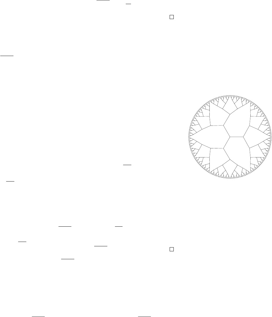
88 ramanujan graphs
and
z
T
Az = x
T
Ax + c
2
y
T
Ay ≥ 2
√
d −1
1 −
1
2r
z
T
z.
Taking r → ∞ as n → ∞ gives the theorem.
We give a second proof of a slightly weaker result, but which is
still in the spirit of Theorem 4.15.
Proof 2 (slightly weaker result). We’ll show that max{|λ
2
|, |λ
n
|} ≥
2
√
d −1 − o(1). This is an illustration of the trace method, also called
the moment method. We have
n
∑
i=1
λ
2k
i
= tr(A
2k
).
The right hand side is the number of closed walks of length 2k on
G. Now, the number of closed walks of length 2k starting at a fixed
vertex v in a d-regular graph is at least the number of closed walks of
length 2k starting at a fixed v in an infinite d-regular tree. To see why
this is true, note that given any walk on the infinite d-regular tree, we
can walk in the same way on G by assigning an orientation to each
vertex. But G may have more walks if it has cycles.
Figure 4.4: Infinite 3-regular tree. Image
taken from the excellent survey on
expander graphs: Shlomo, Linial, and
Wigderson (2006)
There are at least C
k
(d − 1)
k
closed walks of length 2k starting at
a fixed v in an infinite d-regular tree, where C
k
=
1
k+1
(
2k
k
)
is the k-th
Catalan number. Thus, the number of walks of length 2k on G is at
least
n
k+1
(
2k
k
)
(d −1)
k
. On the other hand,
d
2k
+ (n −1)λ
2k
≥
n
∑
i=1
λ
2k
i
.
Thus,
λ
2k
≥
1
k + 1
2k
k
(d −1)
k
−
d
2k
n
.
The term
1
k+1
(
2k
k
)
is (2 − o(1))
2k
as k → ∞. Letting k → ∞ and
k = o(log n) as n → ∞ gives us λ ≥ 2
√
d −1 − o(1).
Remark 4.16. Note that 2
√
d −1 is the spectral radius of the infinite
d-regular tree.
4.5 Ramanujan graphs
10/23: Car l Schildkraut and Milan Haiman
Definition 4.17. A Ramanujan graph is a d-regular graph whose
adjacency matrix has eigenvalues d = λ
1
≥ ··· ≥ λ
n
so that
|
λ
2
|
,
|
λ
n
|
≤ 2
√
d −1, i.e. an (n, d, λ)-graph with λ ≤ 2
√
d −1.
One example of a Ramanujan graph is K
d+1
, as λ
2
= ··· = λ
n
=
−1, but we are more interested in fixing d. For fixed d, do there exist
infinitely many d-regular Ramanujan graphs?

pseudorandom graphs 89
Conjecture 4.18. For all d ≥ 3, there exist infinitely many d-regular
Ramanujan graphs.
We will discuss some partial results towards this conjecture.
Theorem 4.19 (Lubotzky–Phillips–Sarnak, Margulis). The above Lubozsky, Phillips, and Sarnak (1988)
Margulis (1988)
conjecture is true for all d with d −1 prime.
Theorem 4.19 is proven by explicitly constructing a Cayley graph
on the group PSL(2, q) by invoking deep results from number theory
relating to conjectures of Ramanujan, which is where the name comes
from. In 1994, Morgenstern strengthened Theorem 4.19 result to all d Morgenstern (1994)
for which d −1 is a prime power. This is essentially all that is known.
In particular, Conjecture 4.18 is open for d = 7.
It is interesting to consider the case of random graphs. What is the
distribution of the largest non-λ
1
eigenvalue?
Theorem 4.20 (Friedman). Fix d ≥ 3. A random n-vertex d-regular Friedman (2004)
graph is, with prability 1 − o(1) , a nearly-Ramanujan graph in the sense
that
max{
|
λ
2
|
,
|
λ
n
|
} ≤ 2
√
d −1 + o(1)
where the o(1) term goes to 0 as n → ∞ .
Experimental evidence suggests that, for all fixed d, a fixed pro-
portion (between 0 and 1) of graphs on n vertices should be Ramanu-
jan as n → ∞. However, no rigorous results are known in this vein.
Recently, there has been some important progress on a bipartite
analogue of this problem:
Note that for all bipartite graphs, λ
i
= −λ
n+1−i
. To see this, let
the parts be A and B and take an eigenvector v with eigenvalue λ .
Let v consist of v
A
on A and v
B
on B. Then negating v
B
gives an
eigenvector v
0
with eigenvalue −λ. So, a bipartite graph is called
bipartite Ramanujan if λ
2
≤ 2
√
d −1.
G
G ×K
2
An example of a graph G and its
corresponding graph G ×K
2
Every Ramanujan graph G has an associated bipartite Ramanu-
jan graph: we can construct G × K
2
; if G has eigenvalues {λ
i
} then
G × K
2
has eigenvalues {λ
i
} ∪ {−λ
i
}, so the d-regular bipartite Ra-
manujan graph problem is a weakening of the original problem.
Theorem 4.21 (Marcus–Spielman–Srivastava). For all d, there exist Marcus, Spielman, and Srivastava (2015)
infinitely many d-regular bipartite Ramanujan graphs.
Theorem 4.21 uses a particularly clever construction of random-
ized graphs.
4.6 Sparse graph regularity and the Green–Tao theorem
We will now combine the concepts of pseudorandom graphs with
regularity involving sparse graphs. Sparse means edge density o(1)

90 sparse graph regularity and the green–tao theorem
— here we always consider a sequence of graphs on n vertices as
n → ∞, and o(1) is with respect to n. The naïve analogue of the
triangle removal lemma in a sparse setting is not true; we need an
additional constraint:
Meta-Theorem 4.22 (Sparse triangle removal lemma). For all e >
0, there exists δ > 0 so that, if Γ is a sufficiently pseudorandom
graph on n vertices with edge density p and G is a subgraph of Γ
with fewer than δn
3
p
3
triangles, then G can be made triangle-free by
deleting e n
2
p edges.
We call this a meta-theorem as the condition “sufficiently pseu-
dorandom” is not made explicit: the result is precisely true for some
pseudorandomness conditions on which we will elaborate later. We
can consider the traditional triangle removal lemma to be a special
case of this where Γ is a complete graph.
Remark 4.23. Meta-Theorem 4.22 is not true without the hypothesis
of Γ: take G as in Corollary 3.18 to have n vertices and n
2−o(1)
edges,
where every edge belongs to exactly one triangle.
Remark 4.24. If Γ = G(n, p) is an Erd˝os–Rényi graph with p ≥
C
√
n
, Conlon and Gowers (2014)
then the conclusion of Meta-Theorem 4.22 holds.
The motivation for the above is the Green–Tao Theorem:
Theorem 4.25 (Green–Tao). The primes contain arbitrarily long arith- Green and Tao (2008)
metic progressions.
This is in some sense a sparse extension of Szemerédi’s Theorem:
the density of the primes up to n decays like
1
log n
by the Prime Num-
ber Theorem.
The strategy for proving the Theorem 4.25 is to start with the
primes and embed them (with high relative density) in what we will
call pseudoprimes: numbers with no small prime divisors. This set
is easier to analyze with analytic number theory, specifically using
sieve methods. In particular, we can more easily show that the pseu-
doprimes are sufficiently pseudorandom, allowing the use of sparse
hypergraph removal lemmas.
Recall the three main steps of using regularity: partitioning, clean-
ing, and counting. Naïve attempts to apply this approach to prove
the sparse triangle removal lemma result in serious difficulties, and
new ideas are needed. We require a sparse notion of regularity sepa-
rate from the standard notion:
Definition 4.26. Given a graph G, a pair (A, B) ⊂ V(G)
2
is called
(e, p)-regular if, for all U ⊂ A, W ⊂ B with |U| ≥ e|A|, |W| ≥ e|B|,
then
|
d(U, W) − d(A, B)
|
< ep.

pseudorandom graphs 91
An equitable partition V(G) = V
1
t ··· tV
k
is said to be (e, p)-
regular if all but at most e proportion of pairs are (e, p)-regular.
Theorem 4.27 (Sparse regularity lemma). For all e > 0 there exists Scott (2010)
some M ∈ N for which every graph with edge density at most p has an
(e, p)-regular partition into at most M parts.
Sparse objects have in some sense more freedom of structure,
which is why statements like the sparse regularity lemma are much
more intricate than the dense regularity lemma.
Theorem 4.27 is true but quite misleading: it could be true that
most edges are inside irregular pairs. This makes the cleaning step
more difficult as it might clean away too many of your edges. One
example of this is a clique on o(n) vertices.
In practice, G is often assumed to satisfy some “upper-regularity”
hypothesis. For example, a graph is said to have no dense spots if
there exists η = o(1) and a constant C > 0 such that, for all X, Y ⊆
V(G), if |X|, |Y| ≥ η|V|, then
d(X, Y) ≤ Cp.
We will now prove Theorem 4.27 with the “no dense spots” hypothe-
sis:
Proof sketch of Theorem 4.27 under the “no dense spots” hypothesis. This
is essentially the same proof as in Szemerédi’s Regularity Lemma.
The key property we used in the energy increment argument was
that the energy was bounded above by 1 and increased by e
5
. Now
the energy increases by e
5
p
2
. This depends on p, which could break
the proof. However, as there are no dense spots, the final energy is at
most O(C
2
p
2
), so the number of bad steps is bounded (depending on
e).
Theorem 4.27 is still true without the condition “no dense spots,”
however:
0
2
x
Φ
4
Scott’s energy function Φ(x).
Proof sketch of Theorem 4.27 in generality. We repeat the proof of Theo-
rem 3.5 and instead of using x
2
as the energy, consider
Φ(x) =
x
2
if 0 ≤ x ≤ 2
4x −4 if x > 2.
This function has the boosting step: for all random variables X ≥ 0, if
E[X] ≤ 1,
EΦ(X) − Φ
(
EX
)
≥
1
4
Var X.
Furthermore, the inequality
EΦ(X) ≤ 4EX

92 sparse graph regularity and the green–tao theorem
allows us to bound the total energy of a partition by O(1).
Theorem 4.27 shows that the hard part of Meta-Theorem 4.22 is
not the regularity lemma but the counting step. There is no counting
lemma for sparse regular graphs. However, given our hypothesis
that G is a subgraph of a pseudorandom graph Γ, we can construct
a counting lemma which will allow us to prove the sparse triangle
removal lemma.
We want something like the following to be true:
If you have three sets V
1
, V
2
, V
3
so that (V
i
, V
j
) are (e, p)-regular ∀i 6= j
with edge density d
i,j
, the number of triangles with one vertex in each part
is
(
d
12
d
23
d
31
+ O
(
e
c
))
p
3
|V
1
||V
2
||V
3
|.
However, no such statement holds; take G(n, p) with p
1
√
n
and
remove an edge from each triangle.
There is another example, due to Alon:
Example 4.28. There exists a triangle-free pseudorandom d-regular Alon (1995)
graph Γ with d = Θ
n
2/3
that is a (n, d, λ )-graph with λ = Θ
√
d
.
To fix the issues with the above attempt, we have the following
“meta-theorem:”
Meta-Theorem 4.29. Given three sets V
1
, V
2
, V
3
in G where G is a
subgraph of a sufficiently pseudorandom graph with edge density p
so that (V
i
, V
j
) are (e, p)-regular for all i 6= j with edge density d
i,j
,
the number of triangles with one vertex in each part is
(
d
12
d
23
d
31
+ O
(
e
c
))
p
3
|V
1
||V
2
||V
3
|.
We will now create a precise “sufficiently pseudorandom” con-
dition for Meta-Theorem 4.22 and Meta-Theorem 4.29. We say that,
given a graph H, a graph Γ is pseudorandom with respect to H-density if
it has H-density (1 + o(1))p
e(H)
. It turns out that the sparse triangle
counting lemma Meta-Theorem 4.22 holds if Γ is pseudorandom with
respect to H-density for every subgraph H of K
2,2,2
.
H
H
0
H and its 2-blowup H
0
.
Remark 4.30. This condition cannot necessarily be replaced by any of
the other conditions given in Theorem 4.1 as our implication chain
does not hold in a sparse setting.
This plays an analogous role to the C
4
condition in Theorem 4.1;
C
4
was the 2-blowup of an edge, while K
2,2,2
is a 2-blowup of a trian-
gle. This acts somewhat like a graph-theoretic analogue of a second-
moment: controlling copies of a graph H’s second moment allows us
to control copies of H in a subset of V(G).
V
2
V
1
v
V
3
d
12
np
d
13
np
There are not enough vertices to use
(e, p)-regularity.
The proof Theorem 3.13 no longer works in the sparse case. Given
three parts V
1
, V
2
, and V
3
, that are pairwise (e, p)-regular, we can no

pseudorandom graphs 93
longer take the neighbors of a vertex in V
1
that are in V
2
and V
3
and
say that, as there are enough of them, they have enough overlap. This
fails due to the extra factor of p in the sparse case.
Theorem 4.31 (Sparse counting lemma). There exists a sparse counting Conlon, Fox, and Zhao (2015)
lemma for counting H in G ⊂ Γ if Γ is pseudorandom with respect to the
density of every subgraph of the 2-blowup of H.
With this sparse counting lemma, one can prove Meta-Theorem 4.22
with the same proof structure as that of Theorem 3.15, using this
pseudorandom property as our “sufficiently pseudorandom” condi-
tion on Γ.
We state a equivalent version of Roth’s theorem (Theorem 3.19):
Theorem 4.32 (Density Roth’s Theorem). If A ⊂ Z/nZ with |A| =
δn, then A contains at least c(δ)n
2
3-APs where c(δ) > 0 is a constant
depending only on δ.
This can be proven by applying the proof structure from the
proof of Theorem 3.19 using Theorem 3.15 (alternatively, we can
use a supersaturation argument). Similarly to this, we can use Meta-
Theorem 4.22 to prove a sparse analogue of Roth’s Theorem:
Meta-Theorem 4.33 (Relative Roth’s Theorem). If S ⊂ Z/nZ is
sufficiently pseudorandom with |S| = pn, and A ⊂ S with |A| ≥ δ|S|,
then A contains at least c(δ)n
2
p
3
3-APs where c(δ) > 0 is a constant
depending only on δ.
What should “pseudorandom” mean here? Recall our proof of
Roth’s Theorem: creating three copies X, Y, Z of Z/nZ and putting
edges among x ∈ X, y ∈ Y, z ∈ Z if 2x + y ∈ S, x − z ∈ S, −y −
2z ∈ S. From this construction, we can read out the pseudorandom
properties we want this graph Γ
S
to have from our counting lemma.
Z/mZ
Z/mZZ/mZ
y
x
z
x ∼ y iff
2x + y ∈ S
y ∼ z iff
−y −2z ∈ S
x ∼ z iff
x −z ∈ S
Definition 4.34. We say that S ⊂ Z/nZ satisfies a 3-linear-forms
condition if, for uniformly randomly chosen x
0
, x
1
, y
0
, y
1
, z
0
, z
1
∈
Z/nZ, the probability that the twelve numbers formed by the linear
forms corresponding to those above:
−y
0
−2z
0
, x
0
−z
0
, 2x
0
+ y
0
,
−y
1
−2z
0
, x
1
−z
0
, 2x
1
+ y
0
,
−y
0
−2z
1
, x
0
−z
1
, 2x
0
+ y
1
,
−y
1
−2z
1
, x
1
−z
1
, 2x
1
+ y
1
are all in S is within a 1 + o(1) factor of the expectation if S ⊂ Z/nZ
were random with density p, and the same holds for any subset of
these 12 expressions.
We also have a corresponding theorem, a simplification of the
Relative Szemerédi Theorem used by Green–Tao: Green and Tao (2008)
94 sparse graph regularity and the green–tao theorem
Theorem 4.35 (Relative Szemerédi Theorem). Fix k ≥ 3. If S ⊂ Z/nZ Conlon, Fox, and Zhao (2015)
satisfies the k-linear-forms condition then any A ⊂ S with |A| ≥ δ|S| has a
lot of k-APs.
There are still interesting open problems involving sparse regular-
ity, particularly involving what sorts of pseudorandomness hypothe-
ses are required to get counting lemmas.
Remark 4.36. Theorems like Theorem 4.35 can also be proven without
the use of regularity, in particular by using the technique of transfer-
ence: Szemerédi’s Theorem can be treated as a black box, and applied
directly to the sparse setting. For more about this, see “Green–Tao
theorem: an exposition” by Conlon, Fox, Zhao. Conlon, Fox, and Zhao (2014)

5
Graph limits
5.1 Introduction and statements of main results
10/28: Yuan Yao
Graph limits seeks a generalization of analytic limits to graphs. Con-
sider the following two examples that shows the potential parallel
between the set of rational numbers and graphs:
Example 5.1. For x ∈ [0, 1], the minimum of x
3
− x occurs at x =
1/
√
3. But if we restrict ourselves in Q (pretending that we don’t
know about real numbers), a way to express this minimum is to find
a sequence x
1
, x
2
, . . . of rational numbers that converges to 1/
√
3.
Example 5.2. Given p ∈ (0, 1), we want to minimize the density
of C
4
’s among all graphs with edge density p. From Theorem 4.1
we see that the minimum is p
4
, which is obtained via a sequence of
quasirandom graphs. (There is no single finite graph that obtains this
minimum.)
We can consider the set of all graphs as a set of discrete objects
(analogous to Q), and seek its "completion" (analogously R).
Definition 5.3. A graphon ("graph function") is a symmetric measur-
able function W : [0, 1]
2
→ [0, 1] .
Remark 5.4. Definition 5.3 can be generalized to Ω × Ω → [0, 1]
where Ω is any measurable probability space, but for simplicity we
will usually work with Ω = [0, 1]. (In fact, most "nice" measurable
probability space can be represented by [0, 1].)
The codomain of the function can also be generalized to R, in
which case we will refer to the function as a kernel. Note that this
naming convention is not always consistent in literature.
Graphons can be seen as a generalized type of graphs. In fact,
we can convert any graph into a graphon, which allow us to start
imagining what the limits of some sequences of graph should look
like.

96 introduction and statements of main results
Example 5.5. Consider a half graph G
n
, which is a bipartite graph
where one part is labeled 1, 2, . . . , n and the other part is labeled
n + 1, . . . , 2n, and vertices i and n + j is connected if and only if i ≤ j.
If we treat the adjacency matrix Adj(G
n
) as a 0/1 bit image, we can
define graphon W
G
n
: [0, 1]
2
→ [0, 1] (which consists of (2n)
2
"pixels"
of size 1/(2n) × 1/(2n) each). When n goes to infinity, the graphon
converges (pointwise) to a function that looks like Figure 5.2.
1
2
3
4
5
6
7
8
Figure 5.1: The half graph G
n
for n = 4
1
1
2
2
3
3
4
4
5
5
6
6
7
7
8
8
Figure 5.2: The graph of W
G
n
(for
n = 4) and the limit as n goes to infinity
(black is 1, white is 0)
This process of converting graphs to graphons can be easily gener-
alized.
Definition 5.6. Given a graph G with n vertices (labeled 1, . . . , n),
we define its associated graphon as W
G
: [0, 1]
2
→ [0, 1] obtained
by partitioning [0, 1] = I
1
∪ I
2
∪ ··· I
n
with λ(I
i
) = 1/n such that if
(x, y) ∈ I
i
× I
j
, then W(x, y) = 1 if i and j are connected in G and 0
otherwise. (Here λ(I) is the Lebesgue measure of I.)
However, as we experiment with more examples, we see that using
pointwise limit as in Example 5.5 does not suffice for our purpose in
general.
Example 5.7. Consider any sequence of random (or quasirandom)
graphs with edge density 1/2 (with number of vertices approaching
infinity), then the limit (should) approach the constant function W =
1/2, though it certainly does not do so pointwise.
Example 5.8. Consider a complete bipartite graph K
n,n
with the
two parts being odd-indexed and even-indexed vertices. Since the
adjacency matrix looks like a checkerboard, we may expect limit to
look like the 1/2 constant function as well, but this is not the case: if
we instead label the two parts 1, . . . , n and n + 1, . . . 2n, then we see
that the graphons should in fact converge to a 2 × 2 checkerboard
instead.
Figure 5.3: A graph of W
K
n,n
and two
possible limits of W
K
n,n
as n goes to
infinity
The examples above show that we need to (at the very least) take
care of relabeling of the vertices in our definition of graph limits.
Definition 5.9. A graph homomorphism from H to G is a map
φ : V(H) → V(G) such that if uv ∈ E(H) then φ(u)φ(v) ∈ E(G).
(Maps edges to edges.) Let Hom(H, G) be the set of all such homo-
morphisms. and let hom(H, G) = |Hom(H, G)|. Define homomor-
phism density as
t(H, G) =
hom(H, G)
|V(G)|
|V(H)|
.
This is also the probability that a uniformly random map is a homo-
morphism.
Example 5.10. • hom(K
1
, G) = |V(G)|,
graph limits 97
• hom(K
2
, G) = 2|E(G)|,
• hom(K
3
, G) is 6 times the number of triangles in G,
• hom(G, K
3
) is the number of proper 3-colorings of G (where the
colors are labeled, say red/green/blue).
Remark 5.11. Note that the homomorphisms from H to G do not
quite correspond to copies of subgraphs H inside G, because the
homomorphisms can be non-injective. Since the number of non-
injective homomorphisms contribute at most O
H
(n
|V(H)−1|
) (where
n = |V(G)|), they form a lower order contribution as n → ∞ when H
is fixed.
Definition 5.12. Given a symmetric measurable function W : [0, 1]
2
→
R, define
t(H, W) =
Z
[0,1]
|V(H)|
∏
ij∈E(H)
W(x
i
, x
j
)
∏
i∈V(H)
dx
i
.
Note that t(H, G) = t(H, W
G
) for every G and H.
Example 5.13. When H = K
3
, we have
t(K
3
, W) =
Z
[0,1]
3
W(x, y)W(y, z)W(z, x) dxdydz.
This can be viewed as the "triangle density" of W.
We may now define what it means for graphs to converge and
what the limit is.
Definition 5.14. We say that a sequence of graphs G
n
(or graphons
W
n
) is convergent if t(H, G
n
) (or t(H, W
n
)) converges as n goes to
infinity for every graph H. The sequence converges to W if t(H, G
n
)
(or t(H, W
n
)) converges to t(H, W) for every graph H.
Remark 5.15. Though not necessary for the definition, we can think of
|V(G
n
)| going to infinity as n goes to infinity.
A natural question is whether a convergent sequence of graphs has
a "limit". (Spoiler: yes.) We should also consider whether the "limit"
we defined this way is consistent with what we expect. To this end,
we need a notion of "distance" between graphs.
One simple way to define the distance between G and G
0
to be
∑
k
2
−k
|t(H
k
, G) − t(H
k
, G
0
)| for some sequence H
1
, H
2
, . . . of all the
graphs. (Here 2
−k
is added to make sure the sum converges to a
number between 0 and 1.) This is topologically equivalent to the
concept of convergence in Definition 5.14, but it is not useful.
Another possibility is to consider the edit distance between two
graphs (number of edge changes needed), normalized by a factor of
98 introduction and statements of main results
1/|V(G)|
2
. This is also not very useful, since the distance between
any two G(n, 1/2) is around 1/4, but we should expect them to be
similar (and hence have o(1) distance).
This does, however, inspires us to look back to our discussion of
quasirandom graphs and consider when a graph is close to constant
p (i.e. similar to G( n, p)). Recall the DISC criterion in Theorem 4.1,
where we expect |e(X, Y) − p|X||Y|| to be small if the graph is suffi-
ciently random. We can generalize this idea to compare the distance
between two graphs: intuitively, two graphs (on the same vertex set,
say) are close if |e
G
(X, Y) − e
G
0
(X, Y)|/n
2
is small for all subsets X
and Y. We do, however, need some more definitions to handle (for
example) graph isomorphisms (which should not change the dis-
tances) and graphs of different sizes.
Definition 5.16. The cut norm of W : [0, 1]
2
→ R is defined as
kWk
= sup
S,T⊆[0,1]
Z
S×T
W
,
where S and T are measurable sets.
For future reference, we also define some related norms.
Definition 5.17. For W : [0, 1]
2
→ R, define the L
p
norm as
kWk
p
=
(
R
|W|
p
)
1/p
, and the L
∞
norm as the infimum of all the
ream numbers m such that the set of all the points (x, y) for which
W(x, y) > m has measure zero. (This is also called the essential
supremum of W.)
Definition 5.18. We say that φ : [0, 1] → [0, 1] is measure-preserving if
λ(A) = λ(φ
−1
(A)) for all measurable A ⊆ [0, 1].
Example 5.19. The function φ(x) = x + 1/2 mod 1 is clearly measure-
preserving. Perhaps less obviously, φ(x) = 2x mod 1 is also measure-
preserving, since while each interval is dilated by a factor of 2 under
φ, every point has two pre-images, so the two effects cancel out. This
only works because we compare A with φ
−1
(A) instead of φ (A).
Definition 5.20. Write W
φ
(x, y) = W(φ(x), φ(y)) (intuitively, "rela-
belling the vertices"). We define the cut distance
δ
(U, W) = inf
φ
kU −W
φ
k
where φ is a measure-preserving bijection.
For graphs G, G
0
, define the cut distance δ
(G, G
0
) = δ
(W
G
, W
G
0
).
We also define the cut distance between a graph and a graphon as
δ
(G, U) = δ
(W
G
, U).
graph limits 99
Note that φ is not quite the same as permuting vertices: it is al-
lowed to also split vertices or overlay different vertices. This allows
us to optimize the minimum discrepancy/cut norm better than sim-
ply considering graph isomorphisms.
Remark 5.21. The inf in the definition is indeed necessary. Suppose
U(x, y) = xy and W = U
φ
, where φ(x) = 2x mod 1, we cannot attain
kU − W
φ
0
k
= 0 for any φ
0
(although the cut distance is 0) since φ is
not bijective.
Now we present the main theorems in graph limit theory that
we will prove later. First of all, one might suspect that there is an
alternative definition of convergence using the cut distance metric,
but it turns out that this definition is equivalent to Definition 5.14.
Theorem 5.22 (Equivalence of convergence). A sequence of graphs or Borgs, Chayes, Lovász, Sós, and Veszter-
gombi (2008)
graphons is convergent if and only if it is a Cauchy sequence with respect to
the cut (distance) metric.
(A Cauchy sequence with respect to metric d is a sequence {x
i
}
that satisfies sup
m≥0
d(x
n
, x
n+m
) → 0 as n → ∞.)
Theorem 5.23 (Existence of limit). Every convergent sequence of graphs Lovász and Szegedy (2006)
or graphons has a limit graphon.
Denote
˜
W
0
as the space of graphons, where graphons with cut
distance 0 are identified.
Theorem 5.24 (Compactness of the space of graphons). The set
˜
W
0
is Lovász and Szegedy (2007)
a compact metric space under the cut metric.
Remark 5.25. Intuitively, this means that the spaces of "essentially
different" graphs is not very large. This is similar to the regularity
lemma, where every graph has a constant-size description that ap-
proximates the graph well. In fact, we can consider this compactness
theorem as a qualitative analytic version of the regularity lemma.
5.2 W-random graphs
10/30: Car ina Letong Hong
Recall the Erd˝os-Rényi random graphs G(n, p) we’ve seen before. We
now introduce its graphon generalization. Let’s start with a special
case, the stochastic block model. It is a graph with vertices colored
randomly (blue or red), and two red vertices are connected with
probability p
rr
, a red vertex and a blue vertex are connected with
probability p
rb
= p
br
, and two blue vertices are connected with
probability p
bb
.
Definition 5.26. Uniformly pick x
1
, . . . , x
n
from the interval [0, 1]. A
W-random graph, denoted G(n, W), has vertex set [n] and vertices i
and j are connected with probability W(x
i
, x
j
).

100 regularity and counting lemmas
x
2
x
3
x
1
x
1
x
3
x
2
b
r
r
b
∗ ∗
∗ ∗
∗ ∗
Figure 5.4: 2-block model
An important statistical question is that given a graph, whether
there is a good model for where this graph comes from. This gives
some motivation to study W-random graphs. We also learnt that the
sequence of Erd˝os-Rényi random graphs converges to the constant
graphon, where below is an analogous result.
Theorem 5.27. Let W be a graphon. Suppose that for all n, G
n
are chosen
from W-random graphs independently, then G
n
→ W almost surely.
Remark 5.28. In particular, every graphon W is the limit of some se-
quence of graphs. This gives us some form of graph approximations.
The proof for the above theorem uses Azuma’s inequality in order
to show that t(F, G
n
) ≈ t(F, W) with high probability.
5.3 Regularity and counting lemmas
We now develop a series of tools to prove Theorem 5.24.
Theorem 5.29 (Counting Lemma). For graphons W, U and graph F, we
have
|t(F, W) − t(F, U)| ≤ |E(F)| δ
(W, U).
Proof. It suffices to prove |t(F, W) − t(F, U)| ≤ |E(F)|kW − Uk
.
Indeed, by considering the above over U replaced by U
φ
, and taking
the infimum over all measure-preserving bijections φ, we obtain the
desired result.
Recall that the cut norm kWk
= sup
S,T⊆[0,1]
|
R
S×T
W|. Now we
prove its useful reformulation: for measurable functions u and v,
sup
S,T⊆[0,1]
Z
S×T
W
= sup
u,v:[0,1]→[0,1]
Z
[0,1]
2
W(x, y)u(x)v(y)dxdy
.
Here’s the reason for the equality to hold: we take u = 1
S
and v = 1
T
so the left hand side is no more than the right hand side, and then
the bilinearity of the integrand in u, v yields the other direction (the
extrema are attained for u, v taking values at 0 or 1).
We now illustrate the case when F = K
3
. Observe that
t(K
3
, W) − t(K
3
, U) =
Z
((W(x, y)W(x, z)W(y, z) −U(x, y)U(x, z)U(y, z))dxdydz
=
Z
(W −U)(x, y)W(x, z)W(y, z)dxdydz
+
Z
U(x, y) (W −U)(x, z)W(y, z)dxdydz
+
Z
U(x, y)U(x, z)(W −U)(y, z)dxdydz.
Take the first term as an example: for a fixed z,
Z
(W −U)(x, y)W(x, z)W(y, z)dxdydz
≤ kW − Uk

graph limits 101
by the above reformulation. Therefore, the whole sum is bounded by
3kW −Uk
as we desire.
For a general graph F, by the triangle inequality we have
|
t(F, W) −t(F, U)
|
=
Z
(
∏
u
i
v
i
∈E
W(u
i
, v
i
) −
∏
u
i
v
i
∈E
U(u
i
, v
i
))
∏
v∈V
dv
≤
|E|
∑
i=1
Z
i−1
∏
j=1
U(u
j
, v
j
)(W(u
i
, v
i
) −U(u
i
, v
i
))
|E|
∏
k=i+1
W(u
k
, v
k
)
!
∏
v∈V
dv
.
Here, each absolute value term in the sum is bounded by kW −
Uk
the cut norm if we fix all other irrelavant variables (everything
except u
i
and v
i
for the i-th term), altogether implying that |t(F, W) −
t(F, U)| ≤ |E(F)| δ
(W, U).
We now introduce an “averaging function” for graphon W.
Definition 5.30. For a partition P = {S
1
, . . . , S
k
} of [0, 1] into measur-
able subsets, and W : [0, 1]
2
→ R a symmetrical measurable function,
define the stepping operator W
P
: [0, 1]
2
→ R constant on each S
i
×S
j
such that W
P
(x, y) =
1
λ(S
i
)λ(S
j
)
R
S
i
×S
j
W if (x, y) ∈ S
i
×S
j
.
(We ignore the defined term when the denominator equals to 0,
because the sets are measure-zero anyway).
This is actually a projection in Hilbert space L
2
([0, 1]
2
), onto the
subspace of functions constant on each step S
i
× S
j
. It can also be
viewed as the conditional expectation with respect to the σ-algebra
generated by S
i
×S
j
.
Theorem 5.31 (Weak regularity lemma). For any e > 0 and any
graphon W : [0, 1]
2
→ R, there exists a partition P of [0, 1] into no
more than 4
1/e
2
measurable sets such that kW −W
P
k
≤ e.
Definition 5.32. Given graph G, a partition P = {V
1
, . . . , V
k
} of V(G)
is called weakly e-regular if for all A, B ⊂ V(G),
e(A, B) −
k
∑
i,j=1
d(V
i
, V
j
)|A ∩ V
i
||B ∩V
j
|
≤ e|V(G)|
2
.
These are similar but different notions we have seen when intro-
ducing Theorem 3.5.
Theorem 5.33 (Weak Regularity Lemma for Graphs). For all e > 0 Frieze-Kannan (1999)
and graph G, there exists a weakly e-regular partition of V(G) into up to
4
1/e
2
parts.
Lemma 5.34 (L
2
energy increment). Let W be a graphon and P a
partition of [0, 1], satisfying kW − W
P
k
> e. There exists a refine-
ment P
0
of P dividing each part of P into no more than 4 parts, such that
kW
P
0
k
2
2
> kW
P
k
2
2
+ e
2
.

102 regularity and counting lemmas
Proof. Because kW − W
P
k
> e, there exist subsets S, T ⊂ [0, 1]
such that |
R
S×T
(W − W
P
)| > e. Let P
0
be the refinement of P by
introducing S and T (divide P based on whether it’s in S \ T,T \ S,
S ∩ T or S ∩T), and that gives at most 4 sub-parts each.
Define hW, Ui to be
R
WU. We know that hW
P
, W
P
i = hW
P
0
, W
P
i
because W
P
is constant on each step of P, and P
0
is a refinement of
P. Thus, hW
P
0
−W
P
, W
P
i = 0. By Pythagorean Theorem,
kW
P
0
k
2
2
= kW
P
0
−W
P
k
2
2
+ kW
P
k
2
2
> kW
P
k
2
2
+ e
2
,
where the latter inequality comes by the Cauchy–Schwarz inequality,
k1
S×T
k
2
kW
P
0
−W
P
k
2
≥ |hW
P
0
−W
P
, 1
S×T
i| = |hW −W
P
, 1
S×T
i| > e.
Proposition 5.35. For any e > 0, graphon W, and P
0
partition of [0, 1],
there exists partition P refining part of P
0
into no more than 4
1/e
2
parts,
such that kW −W
P
k
≤ e.
This proposition specifically tells us that starting with any given
partition, the regularity argument still works.
Proof. We repeatedly apply Lemma 5.34 to obtain P
0
, P
1
, . . . parti-
tions of [0, 1]. For each step, we either have kW −W
P
k
≤ e and thus
stop, or we know kW
P
0
k
2
2
> kW
P
k
2
2
+ e
2
.
Because kW
P
i
k
2
2
≤ 1, we are guaranteed to stop after fewer than
than e
−2
steps. We also know that each part is subdivided into no
more than 4 parts at each step, obtaining 4
e
−2
as we desire.
We hereby introduce a related result in computer science, the
MAXCUT problem: given a graph G, we want to find max e(S,
¯
S)
among all vertex subsets S ⊂ V(G). Polynomial-time approximation
algorithms developed by Goemans and Williamson that finds a cut Goemans and Williamson (1995)
within around 0.878 fraction of the optimum. conjecture known as Khot, Kindler, Mossel, and O’Donnell
(2007)
the Unique Games Conjecture would imply that the it would not
be possible to obtain a better approximation than the Goemans–
Williamson algorithm.2306295 states the impossibility of beating this.
It is shown that approximating beyond
16
17
≈ 0.941 is NP-hard. Håstad (2001)
On the other hand, the MAXCUT problem becomes easy to ap-
proximate for dense graphs, i.e., approximating the size of the max-
imum cut of an n-vertex graph with in to en
2
additive error in time
polynomial in n, where e > 0 is a fixed constant. One can apply an
algorithmic version of the weak regularity lemma and brute-force
search through all possible partition sizes of the parts. This appli-
cation was one of the original motivations of the weak regularity
lemma.

graph limits 103
5.4 Compactness of the space of graphons
Definition 5.36. A martingale is a random sequence X
0
, X
1
, X
2
, . . .
such that for all n, E[X
n
|X
n−1
, X
n−2
, . . . , X
0
] = X
n−1
.
Example 5.37. Let X
n
denotes the time n balance at a fair casino,
where the expected value of each round’s gain is 0. Then {X
n
}
n≥0
is
a martingale.
Example 5.38. For a fixed random variable X, we define X
n
=
E(X| information up to time n), so that this sequence also forms a
martingale.
Theorem 5.39 (Martingale Convergence Theorem). Every bounded
martingale converges almost surely.
Remark 5.40. Actually, instead of bounded, it is enough for the mar-
tingales to be L
1
-bounded or uniform integrable, both of which gives
sup E(X
+
n
) < ∞.
We sketch a idea inspired by a betting strategy. The proof below
omits some small technical details that can be easily filled in for those
who are familiar with the basic language of probability theory.
•
•
•
•
•
•
•
•
•
•
•
•
a
b
n
•
•
Figure 5.5: examples of “upcrossings”
Proof. An “upcrossing” of [a, b] consists of an interval [n, n + t] such
that X
n
< a, and X
n+t
is the first instance after X
n
such that X
n+t
>
a. We refer to the figure on the right instead of giving a more precise
definition.
Suppose there is a sequence of bounded martingale {X
n
} that
doesn’t converge. Then there exists rational numbers 0 < a < b < 1
such that {X
n
} upcrosses the interval [a, b] infinitely many times. We
will show that this event occurs with probability 0 (so that after we
sum over a, b ∈ Q, {X
n
} converges with probability 1).
Denote u
N
to be the number of upcrossings (crossings from below
to above the interval) up to time N. Consider the following betting
strategy: at any time, we hold either 0 or 1 share. If X
n
< a, then buy
1 share and hold it until the first time that the price (X
n
) reads more
than b (i.e. we sell at time m such that X
m
> b for the first time and
m > n).
How much profit do we make from this betting strategy? We
pocket b − a for each upcrossing. Accounting for difference between
our initial and final balance, our profit is at least (b − a)u
N
− 1. On
the other hand, the optional stopping theorem tells us that every
“fair” betting strategy on a margingale has zero expected profit. So
because the profits of a martingale is zero,
0 = E profit ≥ (b −a)Eu
N
−1,

104 compactness of the space of graphons
which implies Eu
N
≤
1
b−a
. Let u
∞
= lim
N→∞
u
N
denotes the total
number of upcrossings. By the monotone convergence theorem, we
have Eu
∞
≤
1
b−a
too, hence P(u
∞
= ∞) = 0, implying our result.
11/4: Dhr uv Rohatgi
We now prove the main theorems of graph limits using the tools
developed in previous sections, namely the weak regularity lemma
(Theorem 5.31) and the martingale convergence theorem (Theo-
rem 5.39). We will start by proving that the space of graphons is
compact (Theorem 5.24). In the next section we will apply this result
to prove Theorem 5.23 and Theorem 5.22, in that order. We will also
see how compactness can be used to prove a graphon-reformulation
of the strong regularity lemma.
Recall that
e
W
0
is the space of graphons modulo the equivalence
relation W ∼ U if δ
(W, U) = 0. We can see that (
e
W
0
, δ
) is a metric
space.
Theorem 5.41 (Compactness of the space of graphons). The metric Lovász and Szegedy (2007)
space (
e
W
0
, δ
) is compact.
Proof. As
e
W
0
is a metric space, it suffices to prove sequential com-
pactness. Fix a sequence W
1
, W
2
, . . . of graphons. We want to show
that there is a subsequence which converges (with respect to δ
) to
some limit graphon.
For each n, apply the weak regularity lemma (Theorem 5.31) re-
peatedly, to obtain a sequence of partitions
P
n,1
, P
n,2
, P
n,3
, . . .
such that
(a) P
n,k+1
refines P
n,k
for all n, k,
(b) |P
n,k
| = m
k
where m
k
is a function of only k, and
(c)
W
n
−W
n,k
≤ 1/k where W
n,k
= (W
n
)
P
n,k
.
The weak regularity lemma only guarantees that |P
n,k
| ≤ m
k
, but if
we allow empty parts then we can achieve equality.
Initially, each partition may be an arbitrary measurable set. How-
ever, for each n, we can apply a measure-preserving bijection φ to
W
n,1
and P
n,1
so that P
n,1
is a partition of [0, 1] into intervals. For
each k ≥ 2, assuming that P
n,k−1
is a partition of [0, 1] into intervals,
we can apply a measure-preserving bijection to W
n,k
and P
n,k
so that
P
n,k
is a partition of [0, 1] into intervals, and refines P
n,k−1
. By in-
duction, we therefore have that P
n,k
consists of intervals for all n, k.
Properties (a) and (b) above still hold. While property (c) may not
hold, and it’s no longer true that W
n,k
= (W
n
)
P
n,k
, we still know that
δ
(W
n
, W
n,k
) ≤ 1/k for all n, k. This will suffice for our purposes.

graph limits 105
Now, the crux of the proof is a diagonalization argument in count-
ably many steps. Starting with the sequence W
1
, W
2
, . . . , we will
repeatedly pass to a subsequence. In step k, we pick a subsequence
W
n
1
, W
n
2
, . . . such that:
1. the endpoints of the parts of P
n
i
,k
all individually converge as
i → ∞, and
2. W
n
i
,k
converges pointwise almost everywhere to some graphon U
k
as i → ∞.
There is a subsequence satisfying (1) since each partition P
n,k
has
exactly m
k
parts, and each part has length in [0, 1]. So consider a
subsequence (W
a
i
)
∞
i=1
satisfying (1). Each W
a
i
,k
can be naturally iden-
tified with a function f
a
i
,k
: [m
k
]
2
→ [0, 1]. The space of such functions
is bounded, so there is a subsequence ( f
n
i
)
∞
i=1
of ( f
a
i
)
∞
i=1
converging
to some f : [m
k
]
2
→ [0, 1]. Now f corresponds to a graphon U
k
which
is the limit of the subsequence (W
n
i
)
∞
i=1
. Thus, (2) is satisfied as well.
To conclude step k, the subsequence is relabeled as W
1
, W
2
, . . . and
the discarded terms of the sequence are ignored. The corresponding
partitions are also relabeled. Without loss of generality, in step k
we pass to a subsequence which contains W
1
, . . . , W
k
. Thus, the end
result of steps k = 1, 2, . . . is an infinite sequence with the property
that (W
n,k
)
∞
n=1
converges pointwise almost everywhere (a.e.) to U
k
for
all k:
W
1
W
2
W
3
. . .
k = 1 W
1,1
W
2,1
W
3,1
. . . → U
1
pointwise a.e.
k = 2 W
1,2
W
2,2
W
3,2
. . . → U
2
pointwise a.e.
k = 3 W
1,3
W
2,3
W
3,3
. . . → U
3
pointwise a.e.
.
.
.
.
.
.
.
.
.
.
.
.
.
.
.
.
.
.
Similarly, (P
n,k
)
∞
n=1
converges to an interval partition P
k
for all k.
By property (a), each partition P
n,k+1
refines P
n,k
, which implies
that W
n,k
= (W
n,k+1
)
P
n,k
. Taking n → ∞, it follows that U
k
= (U
k+1
)
P
k
(see Figure 5.6 for an example). Now each U
k
can be thought of as
a random variable on probability space [0, 1]
2
. From this view, the
equalities U
k
= (U
k+1
)
P
k
exactly imply that the sequence U
1
, U
2
, . . .
is a martingale.
U
1
0.5
P
1
U
2
0.4
0.6
0.6
0.4
P
2
U
3
0.3 0.4 0.7 0.4
0.4 0.5 0.4 0.9
0.7 0.4 0.4 0.4
0.4 0.9 0.4 0.4
P
3
Figure 5.6: An example of possible U
1
,
U
2
, and U
3
, each graphon averaging the
next.
The range of each U
k
is contained in [0, 1], so the martingale is
bounded. By the martingale convergence theorem (Theorem 5.39),
there exists a graphon U such that U
k
→ U pointwise almost every-
where as k → ∞.
Recall that our goal was to find a convergent subsequence of
W
1
, W
2
, . . . under δ
. We have passed to a subsequence by the above
diagonalization argument, and we claim that it converges to U under

106 applications of compactness
δ
. That is, we want to show that δ(W
n
, U)
→ 0 as n → ∞. This
follows from a standard "3-epsilons argument": let e > 0. Then there
exists some k > 3/e such that
k
U −U
k
k
1
< e/3, by pointwise con-
vergence and the dominated convergence theorem. Since W
n,k
→ U
k
pointwise almost everywhere (and by another application of the
dominated convergence theorem), there exists some n
0
∈ N such that
U
k
−W
n,k
1
< e/3 for all n > n
0
. Finally, since we chose k > 3/e,
we already know that δ(W
n
, W
n,k
)
< e/3 for all n. We conclude that
δ(U, W
n
)
≤ δ(U, U
k
)
+ δ(U
k
, W
n,k
)
+ δ(W
n,k
, W
n
)
≤
k
U −U
k
k
1
+
U
k
−W
n,k
1
+ δ(W
n,k
, W
n
)
≤ e.
The second inequality uses the general bound that
δ(W
1
, W
2
)
≤
k
W
1
−W
2
k
≤
k
W
1
−W
2
k
1
for graphons W
1
, W
2
.
5.5 Applications of compactness
We will now use the compactness of (
e
W
0
, δ
) to prove several results,
notably the strong regularity lemma for graphons, the equivalence of
the convergence criteria defined by graph homomorphism densities
and by the cut norm, and the existence of a graphon limit for every
sequence of graphons with convergent homomorphism densities.
As a warm-up, we will prove that graphons can be uniformly ap-
proximated by graphs under the cut distance. The following lemma
expresses what we could easily prove without compactness:
Lemma 5.42. For every e > 0 and every graphon W, there exists some
graph G such that δ
(G, W) < e.
Proof. By a well-known fact from measure theory, there is a step
function U such that
k
W −U
k
1
< e/2. For any constant graphon p
there is a graph G such that
k
G − p
k
< e/2; in fact, a random graph
G(n, p) satisfies this bound with high probability, for sufficiently
large n. Thus, we can find a graph G such that
k
G −U
k
< e/2 by
piecing together random graphs of various densities. So
δ
(G, W) ≤
k
W −U
k
1
+
k
U − G
k
< e
as desired.
However, in the above lemma, the size of the graph may depend
on W. This can be remedied via compactness.

graph limits 107
Proposition 5.43. For every e > 0 there is some N ∈ N such that for any
graphon W, there is a graph G with N vertices such that δ
(G, W) < e.
Proof. For a graph G, define the e-ball around G by B
e
(G) = {W ∈
e
W
0
: δ
(G, W) < e}.
e
W
0
e
G
Figure 5.7: Cover of
e
W
0
by open balls
As G ranges over all graphs, the balls B
e
(G) form an open cover
of
e
W
0
, by Lemma 5.42. By compactness, this open cover has a fi-
nite subcover. So there is a finite set of graphs G
1
, . . . , G
k
such that
B
e
(G
1
), . . . , B
e
(G
k
) cover
e
W
0
. Let N be the least common multiple of
the vertex sizes of G
1
, . . . , G
k
. Then for each G
i
there is some N-vertex
graph G
0
i
with δ
(G
i
, G
0
i
) = 0, obtained by replacing each vertex of G
i
with N/|V(G
i
)| vertices. But now W is contained in an e-ball around
some N-vertex graph.
Figure 5.8: A K
3
and its 2-blowup. Note
that the graphs define equal graphons.
Remark 5.44. Unfortunately, the above proof gives no information
about the dependence of N on e. This is a byproduct of applying
compactness. One can use regularity to find an alternate proof which
gives a bound.
Intuitively, the compactness theorem has a similar flavor to the
regularity lemma; both are statements that the space of graphs is in
some sense very small. As a more explicit connection, we used the
weak regularity lemma in our proof of compactness, and the strong
regularity lemma follows from compactness straightforwardly.
Theorem 5.45 (Strong regularity lemma for graphons). Let e = Lovász and Szegedy (2007)
(e
1
, e
2
, . . . ) be a sequence of positive real numbers. Then there is some If e
k
= e/k
2
, then this theorem approxi-
mately recovers Szemerédi’s Regularity
Lemma. If e
k
= e, then it approximately
recovers the Weak Regularity Lemma.
M = M(e) such that every graph W can be written
W = W
str
+ W
psr
+ W
sml
where
• W
str
is a step function with k ≤ M parts,
•
W
psr
≤ e
k
,
•
k
W
sml
k
1
≤ e
1
.
Proof. It is a well-known fact from measure theory that any measur-
able function can be approximated arbitrarily well by a step function.
Thus, for every graphon W there is some step function U such that
k
W −U
k
1
≤ e
1
. Unfortunately, the number of steps may depend on
W; this is where we will use compactness.
For graphon W, let k(W) be the minimum k such that some k-
step graphon U satisfies
k
W −U
k
1
≤ e
1
. Then {B
e
k(W)
}
W∈
e
W
0
is
clearly an open cover of
e
W
0
, and by compactness there is a finite set
of graphons S ⊂
e
W
0
such that {B
e
k(W)
(W)}
W∈S
covers
e
W
0
.

108 applications of compactness
Let M = max
W∈S
k(W). Then for every graphon W, there is some
W
0
∈ S such that δ
(W, W
0
) ≤ e
k( W
0
)
. Furthermore, there is a k-step
graphon U with k = k(W
0
) ≤ M such that
k
W
0
−U
k
1
≤ e
1
. Hence,
W = U + (W −W
0
) + ( W
0
−U)
is the desired decomposition, with W
str
= U, W
psr
= W − W
0
, and
W
sml
= W
0
−U.
Earlier we defined convergence of a sequence of graphons in
terms of the sequences of F-densities. However, up until now we
did not know that the limiting F-densities of a convergent sequence
of graphons are achievable by a single graphon. Without completing
the space of graphs to include graphons, this is in fact not true, as we
saw in the setting of quasirandom graphs. Nonetheless in the space
of graphons, the result is true, and follows swiftly from compactness.
Theorem 5.46 (Existence of limit). Let W
1
, W
2
, . . . be a sequence of Lovász and Szegedy (2006)
graphons such that the sequence of F-densities {t(F, W
n
)}
n
converges for
every graph F. Then the sequence of graphons converges to some W. That is,
there exists a graphon W such that t(F, W
n
) → t(F, W) for every F.
Proof. By sequential compactness, there is a subsequence (n
i
)
∞
i=1
and
a graphon W such that δ
(W
n
i
, W) → 0 as i → ∞. Fix a graph F. By
Theorem 5.29, it follows that t(F, W
n
i
) → t(F, W). But by assumption,
the sequence {t(F, W
n
)}
n
converges, so all subsequences have the
same limit. Therefore t(F, W
n
) → t(F, W).
The last main result of graph limits is the equivalence of the two
notions of convergence which we had defined previously.
Theorem 5.47 (Equivalence of convergence). Convergence of F- Borgs, Chayes, Lovász, Sós, and Veszter-
gombi (2008)
densities is equivalent to convergence under the cut norm. That is, let
W
1
, W
2
, . . . be a sequence of graphons. Then the following are equivalent:
• The sequence of F-densities {t(F, W
n
)}
n
converges for all graphs F
• The sequence {W
n
}
n
is Cauchy with respect to δ
.
Proof. One direction follows immediately from Theorem 5.29, the
counting lemma: if the sequence {W
n
}
n
is Cauchy with respect to δ
,
then the counting lemma implies that for every graph F, the sequence
of F-densities is Cauchy, and therefore convergent.
For the reverse direction, suppose that the sequence of F-densities
converges for all graphs F. Let W and U be limit points of {W
n
}
n
(i.e.
limits of convergent subsequences). We want to show that W = U.
Let (n
i
)
∞
i=1
be the subsequence such that W
n
i
→ W. By the count-
ing lemma, t(F, W
n
i
) → t(F, W) for all graphs F, and by conver-
gence of F-densities, t(F, W
n
) → t(F, W) for all graphs F. Similarly,
t(F, W
n
) → t(F, U) for all F. Hence, t(F, U) = t(F, W) for all F.

graph limits 109
By the subsequent lemma, this implies that U = W.
Lemma 5.48 (Moment lemma). Let U and W be graphons such that
t(F, W) = t(F, U) for all F. Then δ
(U, W) = 0. This lemma is named in analogy with
the moment lemma from probability,
which states that if two random vari-
able have the same moments (and are
sufficiently well-behaved) then they are
in fact identically distributed.
Proof. We will sketch the proof. Let G(k, W) denote the W-random
graph on k vertices (see Definition 5.26). It can be shown that for any
k-vertex graph F,
Pr[G(k, W)
∼
=
F as labelled graph] =
∑
F
0
⊇F
(−1)
E(F
0
)−E(F)
t(F
0
, W).
In particular, this implies that the distribution of W-random graphs is
entirely determined by F-densities. So G(k, W) and G(k, U) have the
same distributions.
Let H(k, W) be an edge-weighted W-random graph on vertex
set [ k], with edge weights sampled as follows. Let x
1
, . . . , x
k
∼
Unif([0, 1]) be independent random variables. Set the edge-weight
of (i, j) to be W(x
i
, x
j
).
We claim two facts, whose proofs we omit
• δ
(H(k, W), G(k, W)) → 0 as k → ∞ with probability 1, and
• δ
1
(H(k, W), W) → 0 as k → ∞ with probability 1.
Since G(k, W) and G(k, U) have the same distribution, it follows from
the above facts and the triangle inequality that δ
(W, U) = 0.
A consequence of compactness and the moment lemma is that the
"inverse" of the graphon counting lemma also holds: a bound on F-
densities implies a bound on the cut distance. The proof is left as an
exercise.
Corollary 5.49 (Inverse counting lemma). For every e > 0 there is some
η > 0 and integer k > 0 such that if U and W are graphons with
|t(F, U) − t(F, W)| ≤ η
for every graph F on at most k vertices, then δ
(U, W) ≤ e.
Remark 5.50. The moment lemma implies that a graphon can be
recovered by its F-densities. We might ask whether all F-densities
are necessary, or whether a graphon can be recovered from, say,
finitely many densities. For example, we have seen that if W is the
pseudorandom graphon with density p, then t(K
2
, W) = p and
t(C
4
, W) = p
4
; furthermore, it is uniquely determined by these
densities. If the equalities hold then δ
(W, p) = 0.
The graphons which can be recovered from finitely many F-
densities in this way are called "finitely forcible graphons". Among

110 inequalities between subgraph densities
the graphons known to be finitely forcible are any step function and Lovász and Sós (2008)
the half graphon W(x, y) = 1
x+y≥1
. More generally, W(x, y) = Lovász and Szegedy (2011)
1
p(x,y)≥0
is finitely forcible for any symmetric polynomial p ∈ R[x, y]
which is monotone decreasing on [0, 1].
5.6 Inequalities between subgraph densities
11/6: Olga Medrano Martin del Campo
One of the motivations for studying graph limits is that they provide
an efficient language with which to think about graph inequalities.
For instance, we could be able to answer questions such as the fol-
lowing:
Question 5.51. If t(K
2
, G) = 1/2, what is the minimum possible
value of t(C
4
, G)?
We know the answer to this question; as discussed previously, by
Theorem 4.1 we can consider a sequence of quasirandom graphs;
their limit is a graphon W such that t(K
2
, W) = 2
−4
.
In this section we work on these kind of problems; specifically,
we are interested in homomorphism density inequalities. Two graph
inequaities have been discussed previously in this book; Mantel’s
theorem (Theorem 2.2) and Turán’s theorem (Theorem 2.6):
Theorem 5.52 (Mantel’s Theorem). Let W : [0, 1]
2
→ [0, 1] be a graphon.
If t(K
3
, W) = 0, then t(K
2
, W) ≤ 1/2.
Theorem 5.53 (Turán’s theorem). Let W : [0, 1]
2
→ [0, 1] be a graphon.
If t(K
r+1
, W) = 0, then t(K
2
, W) ≤ 1 −1/r.
Our goal in this section is to determine the set of all feasible edge
density, triangle density pairs for a graphon W, which can be for-
mally written as
D
2,3
= {(t(K
2
, W), t( K
3
, W)) : W graphon } ⊆ [0, 1]
2
.
t(K
3
, W)
t(K
2
, W)
Figure 5.9: Mantel’s Theorem implica-
tion in the plot of D
2,3
(red line)
We know that the limit point of a sequence of graphs is a graphon
(Theorem 5.23), hence the region D
2,3
is closed. Moreover, Mantel’s
Theorem (Theorem 5.52) tells us that the horizontal section of this
region when triangle density is zero extends at most until the point
(1/2, 0) ∈ [0, 1]
2
(see Figure 5.9).
A way in which we can describe D
2,3
is by its cross sections. A
simple argument below shows that each vertical cross section of D
2,3
is a line segment:
Proposition 5.54. For every 0 ≤ r ≤ 1, the set D
2,3
∩[ 0, 1] × {r} is a line
segment with no gaps.

graph limits 111
Proof. Consider two graphons W
0
, W
1
with the same edge density;
then, we can consider
W
t
= (1 − t)W
0
+ tW
1
,
which is a graphon; moreover, its triangle density is mapped contin-
uously as t varies from 0 to 1. Its initial and final values are t(K
3
, W
0
)
and r(K
3
, W
1
), respectively, so every triangle density between these
values can be achieved.
Then, in order to better understand the shape of D
2,3
, we would
like to determine the minimum and maximum subgraph densities
that can be achieved given a fixed edge density. We begin by address-
ing this question:
Question 5.55. What is the maximum number of triangles in an
n-vertex m-edge graph?
The Kruskal–Katona theorem can be
proved using a “compression argu-
ment”: we repeatedly “push” the edges
towards the clique and show that num-
ber of triangles can never decrease in
the process.
An intuitive answer would be that the edges should be arranged
so as to form a clique. This turns out to be the correct answer: a
result known as the Kruskal–Katona theorem implies that a graph
with
(
k
2
)
has at most
(
k
3
)
triangles. Here we prove an slightly weaker
version of this bound.
a
a
1
0
Figure 5.10: Graphon which achieves
upper boundary of D
2,3
: t(K
2
, W) = a
2
and t(K
3
, W) = a
3
Theorem 5.56. For every graphon W : [0, 1]
2
→ [0, 1] ,
t(K
3
, W) ≤ t(K
2
, W)
3/2
.
Remark 5.57. This upper bound is achieved by a graphon like the
one shown in Figure 5.10, which is a limit graphon of a sequence of
cliques in G; for each of these graphons, edge and triangle densities
are, respectively,
t(K
2
, W) = a
2
, t(K
3
, W) = a
3
.
Therefore, The upper boundary of the region D
3,2
is given by the
curve y = x
3/2
, as shown by Figure 5.11.
0.25
0.75
0.5
0.5
0.75
0.75
0
0
1
1
t(K
2
, W)
t(K
3
, W)
Figure 5.11: Plot of upper boundary of
D
2,3
, given by the curve y = x
3/2
in
[0, 1]
2
Proof of Theorem 5.56. It suffices to prove the following inequality for
every graph G:
t(K
3
, G) ≤ t(K
2
, G)
3/2
.
Let us look at hom(K
3
, G) and hom(K
2
, G); these count the number
of closed walks in the graph of length 3 and 2, respectively. These
values correspond to the second and third moments of the spectrum
of the graph G:
hom(K
3
, G) =
k
∑
i=1
λ
3
i
and hom(K
2
, G) =
k
∑
i=1
λ
2
i

112 inequalities between subgraph densities
Where {λ
i
}
n
i=1
are the eigenvalues of the adjacency matrix A
G
. We
then have that
hom(K
3
, G) =
n
∑
i=1
λ
3
i
≤
n
∑
i=1
λ
2
i
!
3/2
= hom(K
2
, G)
3/2
. (5.1)
After dividing by |V(G)|
3
on both sides, the result follows.
Note that in the last proof, we used the following useful inequality,
with a
i
= λ
2
i
and t = 3/2:
Claim 5.58. Let t > 1, and a
1
, ··· , a
n
≥ 0. Then,
a
t
1
+ ··· + a
t
n
≤ (a
1
+ ··· + a
n
)
t
Proof. This inequality is homogeneous with respect to the variables
a
i
, so we can normalize and assume that
∑
a
i
= 1; therefore, each of
the a
i
∈ [0, 1], so that a
t
i
≤ a
i
for each i. Therefore,
LHS = a
t
1
+ ··· + a
t
n
≤ a
1
+ ··· + a
n
= 1 = 1
t
= RHS.
The reader might wonder whether there is a way to prove this
without using eigenvalues of the graph G. We have following result,
whose proof does not require spectral graph theory:
Theorem 5.59. For every W : [0, 1]
2
→ R which is symmetric,
t(K
3
, W) ≤ t(K
2
, W
2
)
3/2
where W
2
corresponds to the graphon W, squared pointwise.
Note that above, t(K
2
, W)
3/2
falls in between these two terms
when W is a graphon because all the terms would be bounded be-
tween 0 and 1; therefore, the above result is stronger than that of
Theorem 5.56. The proof of this result follows from applying the
Cauchy–Schwarz inequality three times; one corresponding to each
edge of a triangle K
3
.
Proof. We have
t(K
3
, W) =
Z
[0,1]
3
W(x, y)W(x, z)W(y, z)dxdydz.
From now on, we drop the notation for our intervals of integration.
We can apply the Cauchy–Schwarz inequality on the following in-
tegral; first with respect to the variable dx, and subsequently with
respect to the variables dy, dz, each time holding the other two vari-

graph limits 113
ables constant:
t(K
3
, W) =
Z
W(x, y)W(x, z)W(y, z)dxdydz
≤
Z
Z
W(x, y)
2
dx
1/2
Z
W(x, z)
2
dx
1/2
W(y, z)dydz
≤
Z
Z
W(x, y)
2
dxdy
1/2
Z
W(x, z)
2
dx
1/2
Z
W(y, z)
2
dy
1/2
dz
≤
Z
W(x, y)
2
dxdy
1/2
Z
W(x, z)
2
dxdz
1/2
Z
W(y, z)
2
dydz
1/2
= kWk
3
2
= t(K
2
, W)
3/2
,
completing the proof.
Remark 5.60. If we did not have the condition that W is symmetric,
we could still use Hölder’s inequality; however, we would obtain a
weaker statement. In this situation, Hölder’s inequality would imply
that
Z
[0,1]
3
f (x, y)g(x, z)h(y, z)dxdydz ≤ kf k
3
kgk
3
khk
3
,
and by setting f = g = h = W, we could derive a weaker bound than
the one obtained in the proof of Theorem 5.59 because, in general,
kWk
2
≤ kWk
3
.
The next theorem allows us to prove linear inequalities between
clique densities.
Theorem 5.61 (Bollobás). Let c
1
, ··· , c
n
∈ R. The inequality Bollobás (1986)
n
∑
r=1
c
r
t(K
r
, G) ≥ 0
holds for every graph G if and only if it holds for every G = K
m
with
m ≥ 1. More explicitly, the inequality holds for all graphs G if and only if
n
∑
r=1
c
r
·
m(m −1) ···(m −r + 1)
m
r
≥ 0
for every m ≥ 1.
Proof. One direction follows immediately because the set of clique
graphs is a subset of the set of all graphs.
We now prove the other direction. The inequality holds for all
graphs if and only if it holds for all graphons, again since the set
of graphs is dense in
f
W
0
with respect to the cut distance metric. In
particular, let us consider the set S of node-weighted simple graphs,
with a normalization
∑
a
i
= 1.
a
2
= 0.1
a
1
= 0.2
a
3
= 0.4
a
4
= 0.3
a
1
a
2
a
3
a
4
a
1
a
2
a
3
a
4
0
1 1 1
1
0 0 0
1
0 0
1
1
0
1
0
Figure 5.12: Example of a node
weighted graph on four vertices, whose
weights sum to 1, and its corresponding
graphon.
114 inequalities between subgraph densities
As Figure 5.12 shows, each node weighted graph can be repre-
sented by a graphon. The set S is dense in
f
W
0
, because this set con-
tains the set of unweighted simple graphs. Then, it suffices to prove
this inequality for graphs in S.
Suppose for the sake of contradiction that there exists a node
weighted simple graph H such that
f (H) :=
n
∑
r=1
c
r
t(K
r
, H) < 0
Among all such H, we choose one with smallest possible number m
of nodes. We choose node weights a
1
, ··· , a
m
with sum equal to 1
such that f (H) is minimized. We can find such H because we have
a finite number of parameters, and f is a continuous function over a
compact set.
We have that a
i
> 0 without loss of generality; otherwise we
would have a contradiction because we could delete that node and
decrease the quantity |V(H)|, while f (H) < 0 would still hold.
Moreover, H is a complete graph; otherwise there exist i, j such
that ij 6∈ E(H) . Note that the clique density is a polynomial in terms
of the node weights; this polynomial would not have an a
2
i
term
because the set of graphons S corresponds to simple graphs, and
the vertex i would not be adjacent to itself. This polynomial does not
have an a
i
a
j
term either, because i and j are not adjacent. Therefore,
f (H) is multilinear in the variables a
i
and a
j
.
Fixing all of the other node weights and considering a
i
, a
j
as our
variables of the multilinear function f (H), this function would be
minimized by setting a
i
= 0 or a
j
= 0. If one of these weights were
set to zero, this would imply a decrease in the number of nodes,
while a
i
+ a
j
would be preserved, hence not increasing f (H) . This is
a contradiction to the minimality of number of nodes in H such that
f (H) < 0.
In other words, H must be a complete graph; further, the polyno-
mial f (H) on the variables a
i
has to be symmetric:
f (H) =
n
∑
r=1
c
r
r!s
r
,
where each s
r
is an elementary symmetric polynomial of degree r
s
r
=
∑
i
1
<···<i
r
a
i
1
···a
i
r
.
In particular, by making constant all variables but a
1
, a
2
, the polyno-
mial f (H) can be written as
f (H) = A + B
1
a
1
+ B
2
a
2
+ Ca
1
a
2
,

graph limits 115
where A, B
1
, B
2
, C are constants; by symmetry, we have B
1
= B
2
; also,
since
∑
a
i
= 1, we have that a
1
+ a
2
is constant, so that
f (H) = A
0
+ Ca
1
a
2
.
If C > 0 then f would be minimized when a
1
= 0 or a
2
= 0; this
cannot occur because of the minimality of the number of nodes in
H. If C = 0 then any value of a
1
, a
2
would yield the same minimum
value of f (H); in particular we could set a
1
= 0, again contradicting
minimality on the number of nodes. Therefore, the constant C must
be negative,implying that f (H) would be minimized when a
1
= a
2
.
Then, all of the a
i
have to be equal, and H can also be regarded as an
unweighted graph.
In other words, if the inequality of interest fails for some graph H,
then it must fail for some unweighted clique H; this completes the
proof.
Remark 5.62. In the proof above, we only considered clique densities;
an inequality over other kinds of graphs would not necessarily hold.
Thanks to the theorem above, it is relatively simple to test linear
inequalities between densities, since we just have to verify them for
cliques. We have the following corollary:
Corollary 5.63. For each n, the extremal points of the convex hull of
{( (t(K
2
, W), t( K
3
, W), ··· , t(K
n
, W)) : W graphon} ⊂ [0, 1]
n−1
are given by W = K
m
for all m ≥ 1.
Note that the above claim implies Turán’s theorem, because by
Theorem 5.61, the extrema of the set above are given in terms of
clique densities, which can be understood by taking W to be a clique.
Thus, if t(K
r+1
, W) = 0, then this cross section on the higher dimen-
sional cube [0, 1]
r
will be bounded by the value t(K
2
, W) = 1 −
1
r
.
In the particular case that we want to find the extremal points in
the convex hull of D
2,3
⊂ [0, 1]
2
, they correspond to
p
m
=
m −1
m
,
(m −1)(m −2)
m
2
All of the points of these form in fact fall into the curve given by
y = x(2x −1), which is the dotted red curve in Section 5.6.
1
2
0
2
3
2/9
3
4
3/8
4
5
12/25
5
6
5/9
.
.
.
···
t(K
2
, W)
t(K
3
, W)
Figure 5.13: Set of lower boundary
points of D
2,3
, all found in the curve
given by y = x(2x −1)
Because the region D
2,3
is contained in the convex hull of the red
points {p
m
}
m≥0
, it also lies above the curve y = x(2x − 1). We can
moreover draw line segments between the convex hull points, so as
to obtain a polygonal region that bounds D
2,3
.
The region D
2,3
was determined by Razborov, who developed the
Razborov (2007)
theory of flag algebras, which have provided a useful framework in
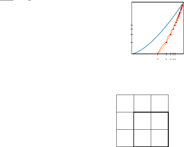
116 inequalities between subgraph densities
which to set up sum of squares inequalities, e.g., large systematic
applications of the Cauchy–Schwarz inequalities, that could be used
in order to prove graph density inequalities.
Theorem 5.64 (Razborov). For a fixed edge density t(K
2
, W), which falls Razborov (2008)
into the following interval, for some k ∈ N
t(K
2
, W) ∈
1 −
1
k − 1
, 1 −
1
k
,
the minimum feasible t(K
3
, W) is attained by a unique step function
graphon corresponding to a k-clique with node weights a
1
, a
2
, ··· , a
k
with
sum equal to 1, and such that a
1
= ··· = a
k−1
≥ a
k
.
1
2
0
2
3
2/9
3
4
3/8
4
5
12/25
5
6
5/9
.
.
.
···
t(K
2
, W)
t(K
3
, W)
Figure 5.14: Complete description of the
region D
2,3
⊂ [0, 1]
2
The region D
2,3
is illustrated on the right in Section 5.6. We have
exaggerated the drawwings of the concave “scallops” in the lower
boundary of the region for better visual effects.
Note that in Turán’s theorem, the construction for the graphs
which correspond to extrema value (Chapter 2, definition 2.5) are
unique; however, in all of the intermediate values t(t
2
, W) 6= 1 −1/k,
this theorem provides us with non-unique constructions.
To illustrate why these constructions are not unique, the graphon
in Figure 5.15, which is a minimizer for triangle density when t(t
2
, W) =
2/3 can be modified by replacing the highlighted region by any
graphon with the same edge density.
α
1
α
2
α
3
α
1
α
2
α
3
1 1
0
1
0
1
0
1 1
Figure 5.15: A non unique optimal
graphon in the case k = 3.
Non-uniqueness of graphons that minimize t(K
3
, W) implies that
this optimization problem is actually difficult.
The problem of minimizing the K
r
-density in a graph of given
edge density was solved for r = 4 by Nikiforov and all r by Reiher.,
Nikiforov (2011)
Reiher (2016)
respectively.
More generally, given some inequality between various subgraph
densities, can we decide if the inequality holds for all graphons?
For polynomial inequalities between homomorphism densities, it
suffices to only consider linear densities, since t(H, W)t(H
0
, W) =
t(H t H
0
, W).
Let us further motivate with a related, more classical question
regarding nonnegativity of polynomials:
Question 5.65. Given a multivariable polynomial p ∈ R[x
1
, x
2
, ··· , x
n
],
is p(x) ≥ 0 for every x = (x
1
, ··· , x
n
)?
This problem is decidable, due to a classic result of Tarski that
every the first-order theory of the reals is decidable. In fact, we have
the following characterization of nonnegative real polynomials.
Theorem 5.66 (Artin). A polynomial p ∈ R[x
1
, x
2
, ··· , x
n
] is nonnega-
tive if and only if it can be written as a sum of squares of rational functions.
graph limits 117
However, when we turn our interest into the set of lattice points,
the landscape changes:
Question 5.67. Given a multivariable polynomial p ∈ R[x
1
, x
2
, ··· , x
n
],
can it be determined whether p(x
1
, ··· , x
n
) ≥ 0 for all x ∈ Z
n
?
The answer to the above question is no. This is related to the fact
that one cannot solve diophantine equations, or even tell whether
there is a solution:
Theorem 5.68 (Matiyasevich; Hilbert’s 10th problem). Given a gen- Matiyasevich (2011)
eral diophantine equation is an undecidable problem to find its solutions, or
even to determine whether integer solutions exist.
Turning back to our original question of interest, we want to know
whether the following question is decidable
Question 5.69. For a given set of graphs {H
i
}
i∈[k]
and a
1
, ··· , a
k
∈ R,
is
∑
k
i=1
a
i
t(H
i
, G) ≥ 0 true for every graph G?
The following theorem provides an answer to this question:
Theorem 5.70 (Hatami - Norine). Given a set of graphs {H
i
}
i∈[k]
and Hatami and Norine (2011)
a
1
, ··· , a
k
∈ R, whether the inequality
k
∑
i=1
a
i
t(H
i
, G) ≥ 0
is true for every graph G is undecidable.
A rough intuition for why the above theorem is true is that we
actually have a discrete set of points along the lower boundary of
D
2,3
; one could reduce the above problem into proving the same in-
equalities along the points in the intersection of the red curve and the
region. The set of points in this intersection forms a discrete set, and
the idea is to encode integer inequalities (which are undecidable) into
graph inequalities by using the special points on the lower boundary
of D
2,3
.
Another kind of interesting question is to ask whether specific
inequalities are true; there are several open problems of that type.
Here is an important conjecture in extremal graph theory:
Conjecture 5.71 (Sidorenko’s Conjecture). If H is a bipartite graph then Sidorenko (1993)
t(H, W) ≥ t(K
2
, W)
e(H)
.
We worked recently with an instance of the above inequality, when
H = C
4
, when we were discussing quasirandomness. However,
the above problem is open. Let us consider the Möebius strip graph
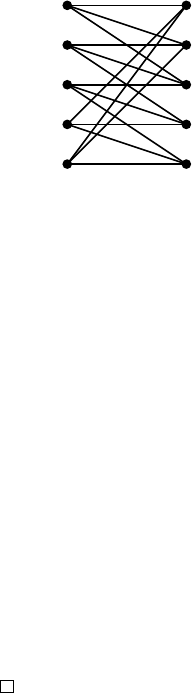
118 inequalities between subgraph densities
- which consists in removing a 10-cycle from a complete bipartite
graph K
5,5
(Section 5.6).
The name of this graph comes from its realization as a face-vertex
incidence graph of the usual simplicial complex of the Möebius strip.
The graph above is the first one for which this inequality remains an
open problem.
Figure 5.16: The Möebius strip graph.
Even if nonnegativeness of a general linear graph inequalities is
undecidable, if one wants to decide whether they are true up to an
ε-error, the problem becomes more accessible:
Theorem 5.72. There exists an algorithm that, for every ε > 0 decides
correctly that
n
∑
i=1
c
i
t(H
i
, G) ≥ −ε
for all graphs G, or outputs a graph G such that
n
∑
i=1
c
i
t(H
i
, G) < 0.
Proof sketch. As a result of weak regularity lemma, we can take a
weakly ε-regular partition. All the information regarding edge den-
sities can be represented by this partition; in other words, one would
only have to test a bounded number of possibilities on weighted
node graphs with ≤ M(ε) parts whose edge weights are multiples
of ε. If the estimate for the corresponding weighted sum of graph
densities is true for the auxiliary graph one gets from weak regular-
ity lemma, then it is also true for the original graph up to an ε -error;
otherwise, we can output a counterexample.
Part II
Additive combinatorics

6
Roth’s theorem
11/13: Dain Kim and Anqi Li
In Chapter 3.3, we proved Roth’s theorem using Szemerédi regularity
lemma via the triangle removal lemma. In this chapter, we will be
instead be studying Roth’s original proof of Roth’s Theorem using
Fourier analysis. First, let us recall the statement of Roth’s Theorem.
Let r
3
([N]) denote the maximum size of a 3-AP-free subset of [N].
Then Roth’s theorem states that r
3
([N]) = o(N).
One of the drawbacks of using Szemerédi regularity which shows
an upper bound that is something like
N
log
∗
N
. Roth’s Fourier ana-
lytic proof would instead give us an upper bound of something like
N
log log N
, which is a much more reasonable bound.
Sanders (2011)
Bloom (2016)
Remark 6.1. The current best upper bound known is r
3
([N]) ≤
N(log N)
1−o(1)
and the best lower bound known is r
3
(N) ≥ Ne
−O(
√
log N)
due to the Behrend construction. There is some evidence that seem to
suggest that the lower bound is closer to truth, but closing the gap is
still an open problem.
6.1 Roth’s theorem in finite fields
We will begin by examining a finite field analogue to Roth’s The-
orem. Finite field models are a good sandbox for testing methods
before applying to general integer cases; in particular, it is a good
starting point because a lot of technicalities go away.
Let r
3
(F
n
3
) denote the maximum size of 3 AP-free subset of F
n
3
.
Note that given x, y, z in F
n
3
, the following are equivalent:
• x, y, z for a 3 term arithmetic progression
• x −2y + z = 0
• x + y + z = 0
• x, y, z form a line

122 roth’s theorem in finite fields
• for all i, the ith coordinate of x, y, z are all distinct or all equal. This is relevant to the game of SET,
which can be thought of as finding 3
APs in F
4
3
.
We will state and prove a version of Roth’s theorem in the finite
field model. The proof is in the same spirit as the general Roth’s
theorem, but is slightly easier.
Meshulam (1995)
Theorem 6.2.
r
3
(F
n
3
) = O
3
n
n
The proof using triangle removal lemma copies verbatim so we
can get r
3
(F
n
3
) = o
(
3
n
)
but the above theorem gives a better depen-
dence.
We comment briefly on the history of this problem. In 2004, Edel Edel (2004)
found that r
3
(F
n
3
) ≥ 2.21
n
. It was open for a long time whether
r
3
(F
n
3
) = (3 − o(1))
n
. Recently, a surprising breakthrough showed
that r
3
(F
n
3
) ≤ 2.76
n
. Croot, Lev, Pach (2016)
Ellenberg and Gijswijt (2016)
We had an energy increment argument during the proof of Sze-
merédi Regularity lemma. The strategy for Roth’s theorem is a vari-
ant of energy increment. Instead, we will consider density increment.
Given A ⊂ F
n
3
, we employ the follow strategy.
1. If A is pseudorandom (which we will see is equivalent to it being
Fourier uniform, which roughly translates to all its Fourier coeffi-
cients are small) then there is a counting lemma which will show
that A has lots of 3-AP.
2. If A is not pseudorandom, then we will show that A has a large
Fourier coefficient. Then we can find a codimension 1 affine sub-
space (i.e. hyperplane) where density of A will increase. Now we
consider A restricted to this hyperplane, and repeat the previous
steps.
3. Each time we repeat, we obtain a density increment. Since density
is bounded above by 1, this gives us a bounded number of steps.
Next, we recall some Fourier analytic ideas that will be important
in our proof. In F
n
3
, we consider the Fourier characters γ
r
: F
n
3
→ C,
indexed by r ∈ F
n
3
, which are defined to be γ
r
(x) = ω
r·x
where ω =
e
2πi/3
and r · x = r
1
x
1
+ ··· + r
n
x
n
. We define a Fourier transform.
For f : F
n
3
→ C, the Fourier transform is given by
b
f : F
n
3
→ C where
b
f (r) =
E
x∈F
n
3
f (x)ω
−r·x
= hf , γ
r
i.
Effectively, the fourier transform is the inner product of f and the
Fourier characters.

roth’s theorem 123
Remark 6.3. We use the following convention on normalization: in a
finite group, for a physical space we will use average measure but in
frequency we will always use sum measure.
We note some key properties of the Fourier transform.
Proposition 6.4. •
b
f (0) =
E
f
• (Plancheral/Parseval)
E
x∈F
n
3
f (x)g(x) =
∑
r∈F
n
3
b
f (r)
b
g(r).
• (Inversion) f (x) =
∑
r∈F
n
3
b
f (r)ω
r·x
• (Convolution) Define ( f ∗ g)(x) =
E
y
f (y)g(x −y). Then we claim that
[
f ∗ g(x) =
b
f (x)
b
g(x).
To prove these properties notice that Fourier characters form an
orthonormal basis. Indeed, we can check
hγ
r
, γ
s
i =
E
x
γ
r
(x)γ
s
(x) =
E
x
ω
−(r−s)·x
=
1 if r = s,
0 otherwise.
If we think of Fourier transform as a unitary change of basis, in-
version and Parseval’s follows immediately. To see the formula for
convolution, note that
E
x
( f ∗g)ω
r·x
=
E
x,y
f (y)g(x −y)ω
−r(y+(x−y))
=
E
r
f (x)ω
−r·x
E
s
g(x)ω
−s·x
.
The following key identity relates Fourier transform with 3-APs.
Proposition 6.5. If f , g, h : F
n
3
→ C, then
E
x,y
f (x)g(x + y)h(x + 2y) =
∑
r
b
f (r)
b
g(−2r)
b
h(r).
We will give two proofs of this proposition, with the second being
more conceptual.
First proof. We expand the LHS using the formula for Fourier inver-
sion.
LHS =
E
x,y
∑
r
1
b
f (r
1
)ω
r
1
·x
!
∑
r
2
b
g(r
2
)ω
r
2
·(x+y)
!
∑
r
3
b
h(r
3
)ω
r
3
·(x+2y)
!
=
∑
r
1
,r
2
,r
3
b
f (r
1
)
b
g(r
2
)
b
h(r
3
)
E
x
ω
x·(r
1
+r
2
+r
3
)
E
y
ω
y·(r
2
+2r
3
)
=
∑
r
b
f (r)
b
g(−2r)
b
h(r)
The last equality follows because
E
x
ω
x·(r
1
+r
2
+r
3
)
=
1 if r
1
+ r
2
+ r
3
= 0,
0 otherwise

124 roth’s theorem in finite fields
and
E
y
ω
y·(r
2
+2r
3
)
=
1 if r
2
+ 2r
3
= 0,
0 otherwise.
Second proof. In this proof, we think of the LHS as a convolution.
E
x,y,z:x+y+z=0
f (x)g(y)h(z) = ( f ∗ g ∗h)(0)
=
∑
r
\
f ∗ g ∗ h(r)
=
∑
r
b
f (r)
b
g(r)
b
h(r)
In particular, note that if we take f , g, h = 1
A
where A ⊂ F
n
3
, then
3
−2n
#{(x, y, z) ∈ A
3
: x + y + z = 0} =
∑
r
b
1
A
(r)
3
. (6.1)
Remark 6.6. If A = −A then this gives the same formula that counts
closed walks of length 3 in Cayley graphs. In particular, {
b
1
A
(r) = r}
correspond eigenvalues of Cayley(G, A).
Lemma 6.7 (Counting Lemma). If A ⊂ F
n
3
with |A| = α3
n
, let
Λ
3
(A) =
E
x,y
1
A
(x)1
A
(x + y)1
A
(x + 2y). Then,
Λ
3
(A) − α
3
≤ α max
r6=0
c
1
A
(r)
.
Proof. By Proposition 6.5,
Λ
3
(A) =
∑
r
c
1
A
(r)
3
= α
3
+
∑
r6=0
c
1
A
(r)
3
.
Therefore,
Λ
3
(A) − α
3
≤
∑
r6=0
c
1
A
(r)
3
≤ max
r6=0
c
1
A
(r)
·
∑
r
c
1
A
(r)
2
= max
r6=0
c
1
A
(r)
·E1
2
A
(Parseval)
= α max
r6=0
c
1
A
(r)
.
Proof of Theorem 6.2. Let N = 3
n
, the number of elements in F
n
3
.
Step 1. If the set is 3-AP free, then there is a large Fourier coefficient.
Lemma 6.8. If A is 3-AP-free and N ≥ 2α
−2
, then there is r 6= 0 such that
c
1
A
(r)
≥ α
2
/2.

roth’s theorem 125
Proof. By counting lemma and the fact that Λ
3
(A) =
|A|
N
2
=
α
N
,
α max
r6=0
c
1
A
(r)
≥ α
3
−
α
N
≥
α
3
2
.
Step 2. Large Fourier coefficient implies density increment on a hyper-
plane.
Lemma 6.9. If
c
1
A
(r)
≥ δ for some r 6= 0, then A has density at least
α +
δ
2
when restricted to some hyperplane.
Proof. We have
c
1
A
(r) =
E
x∈F
n
3
1
A
(x)w
−r·x
=
1
3
(α
0
+ α
1
w + α
2
w
2
)
where α
0
, α
1
, α
2
are densities of A on the cosets of r
⊥
. Notice that
α =
α
0
+α
1
+α
2
3
. By triangle inequality,
3δ ≤
α
0
+ α
1
w + α
2
w
2
=
(α
0
−α) + (α
1
−α)w + (α
2
−α)w
2
≤
2
∑
j=0
|α
j
−α|
≤
2
∑
j=0
(|α
j
−α| + (α
j
−α)).
(This final step is a trick that will be useful in the next section.) Note
that every term in the last summation is non-negative. Consequently,
there exists j such that δ ≤ |α
j
−α| + (α
j
−α). Then, α
j
≥ α +
δ
2
.
Step 3 : Iterate density increment.
So far, we have that if A is 3-AP-free and N ≥ 2α
−2
, then A has
density at least α + α
2
/4 on some hyperplane. Let our initial density
be α
0
= α. At the i-th step, we restrict A to some hyperplane, so that
the restriction of A inside the smaller space has density
α
i
≥ α
i−1
+ α
2
i−1
/4.
Let N
i
= 3
n−i
. We can continue at step i as long as N
i
≥ 2α
−2
i
.
We note that the first index i
1
such that α
i
1
≥ 2α
0
satisfies i
1
≤
4
α
+ 1. This is because α
i+1
≥ α + i
α
2
4
. Similar calculations shows that
if i
`
is the first index such that α
i
`
≥ 2
`
α
0
then
i
`
≤
4
α
+ m
2
α
+ ··· +
4
2
`−1
α
+ ` ≤
8
α
+ log
2
1
α
.

126 roth’s proof of roth’s theorem in the integers
Suppose the process terminates after m steps with density α
m
.
Then we find that the size of the subspace in the last step is given by
3
n−m
< 2α
−2
m
≤ 2α
−2
. So
n ≤
8
α
+ log
3
2
α
2
= O
1
α
Thus
|A|
N
= α = O(1/n). Equivalently, |A| = αN = O
3
n
n
as
desired.
Remark 6.10. This proof is much more difficult in integers, because
there is no subspace to pass down to.
11/18: Eshaan Nichani
A natural question is whether this technique can be generalized to
bound 4-AP counts. In the regularity-based proof of Roth’s theorem,
we saw that the graph removal lemma was not sufficient, and we
actually needed hypergraph regularity and a hypergraph removal
lemma to govern 4-AP counts. Similarly, while the counting lemma
developed here shows that Fourier coefficients control 3-AP counts,
they do not in fact control 4-AP counts. For example, consider the
set A = {x ∈ F
n
5
: x · x = 0}. One can show that the nonzero
Fourier coefficients corresponding to A are all small. However, one
can also show that A has the wrong number of 4-APs, thus implying
that Fourier coefficients cannot control 4-AP counts. The field of
higher-order Fourier analysis, namely quadratic Fourier analysis,
was developed by Gowers specifically to extend this proof of Roth’s
Theorem to prove Szemeredi’s Theorem for larger APs. An example Gowers (1998)
of quadratic Fourier analysis is given by the following theorem.
Theorem 6.11 (Inverse theorem for quadratic Fourier analysis). For all
δ > 0, there exists a constant c(δ) > 0 such that if A ⊂ F
n
5
has density α,
and |Λ
4
(A) − α
4
| > δ, then there exists a non-zero quadratic polynomial
f (x
1
, . . . , x
n
) over F
5
satisfying
|E
x∈F
n
5
1
A
(x)ω
f (x)
| ≥ c(δ).
6.2 Roth’s proof of Roth’s theorem in the integers
In Section 6.1 we saw the proof of Roth’s theorem in the finite field
setting, specifically for the set F
n
3
. We will now extend this analysis to
prove the following bound, which will imply Roth’s theorem in the
integers:
Theorem 6.12. Roth (1953)
r
3
([N]) = O
N
log log N
.

roth’s theorem 127
The subsequent proof of this bound is the original one given by
Roth himself. Recall that the proof of Roth’s theorem in finite fields
had the following 3 steps:
1. Show that a 3-AP-free set admits a large Fourier coefficient.
2. Deduce that there must exist a subspace with a density increment.
3. Iterate the density increment to upper bound the size of a 3-AP
free set.
The proof of Roth’s theorem on the integers will follow the same 3
steps. However, the execution will be quite different. The main differ-
ence lies in step 2, where there is no obvious notion of a subspace of
[N].
Previously we defined Fourier analysis in terms of the group F
n
3
.
There is a general theory of Fourier analysis on Abelian groups
which relates a group G to its set of characters
b
G, also referred to
as its dual group. For now, however, we work with the group Z.
The dual group of Z is
b
Z = R/Z. The Fourier Transform of a
function f : Z → C is given by the function
b
f : R/Z → C satisfying
b
f (θ) =
∑
x∈Z
f (x)e(−xθ),
where e(t) = e
2πit
. This is commonly referred to as the Fourier series
of f .
As they were in F
n
3
, the following identities are also true in Z.
Their proofs are the same.
•
b
f (0) =
∑
x∈Z
f (x)
• (Plancherel/Parseval)
∑
x∈Z
f (x)g(x) =
R
1
0
b
f (θ)
b
g(θ)dθ
• (Inversion) f (x) =
R
1
0
b
f (θ)e(xθ)dθ
• Define Λ( f , g, h) =
∑
x,y∈Z
f (x)g(x + y)h(x + 2y). Then
Λ( f , g, h) =
Z
1
0
b
f (θ)
b
g(−2θ)
b
h(θ)dθ.
In the finite field setting, we defined a counting lemma, which
showed that if two functions had similar Fourier transforms, then
they had a similar number of 3-APs. We can define an analogue to
the counting lemma in Z as well.
Theorem 6.13 (Counting Lemma). Let f , g : Z → C such that
∑
n∈Z
|f (n)|
2
,
∑
n∈Z
|g(n)|
2
≤ M. Define Λ
3
( f ) = Λ( f , f , f ). Then
|Λ
3
( f ) − Λ
3
(g)| ≤ 3M
[
f − g
∞
.

128 roth’s proof of roth’s theorem in the integers
Proof. We can rewrite
Λ
3
( f ) − Λ
3
(g) = Λ( f − g, f , f ) + Λ(g, f − g, f ) + Λ(g, g, f − g).
We want to show that each of these terms is small when f − g has
small Fourier coefficients. We know that
|Λ( f − g, f , f )| =
Z
1
0
\
( f − g)(θ)
b
f (−2θ)
b
f (θ)dθ
≤
[
f − g
∞
Z
1
0
b
f (−2θ)
b
f (θ)dθ
(triangle inequality)
≤
[
f − g
∞
Z
1
0
|
b
f (−2θ)|
2
dθ
1/2
Z
1
0
|
b
f (θ)|
2
dθ
1/2
(Cauchy-Schwarz)
≤
[
f − g
∞
∑
x∈Z
|f (x)|
2
!
(Plancherel)
≤ M
[
f − g
∞
.
Bounding the other two terms is identical.
We can now proceed with proving Roth’s Theorem.
Proof of Theorem 6.12. We follow the same 3 steps as in the finite field
setting.
Step 1: 3-AP free sets induce a large Fourier coefficient
Lemma 6.14. Let A ⊂ [N] be a 3-AP free set, |A| = αN, N ≥ 5/α
2
. Then
there exists θ ∈ R satisfying
N
∑
n=1
(1
A
−α)(n)e(θn)
≥
α
2
10
N
Proof. Since A has no 3-AP, the quantity 1
A
(x)1
A
(x + y)1
A
(x + 2y) is
nonzero only for trivial APs, i.e. when y = 0. Thus Λ
3
(1
A
) = |A| =
αN. Now consider Λ
3
(1
[N]
). This counts the number of 3-APs in [N].
We can form a 3-AP by choosing the first and third elements from
[N], assuming they are the same parity. Therefore Λ
3
(1
[N]
) ≥ N
2
/2.
Now, we apply the counting lemma to f = 1
A
, g = α1
[N]
Remark 6.15. The spirit of this whole proof is the theme of structure
versus pseudorandomness, an idea we also saw in our discussion
graph regularity. If A is “pseudorandom”, then we wish to show that
A has small Fourier coefficients. But that would indicate that f and
g have similar Fourier coefficients, implying that A has many 3-AP
counts, which is a contradiction. Thus A cannot be pseudorandom, it
must have some structure.

roth’s theorem 129
Applying Theorem 6.13 yields (where we use the notation f
∧
=
b
f )
α
3
N
2
2
−αN ≤ 3αN
(1
A
−α1
[N]
)
∧
∞
and thus
(1
A
−α1
[N]
)
∧
∞
≥
1
2
α
3
N
2
−αN
3αN
=
1
6
α
2
N −
1
3
≥
1
10
α
2
N,
where in the last inequality we used the fact that N ≥ 5/α
2
. There-
fore there exists some θ with
N
∑
n=1
(1
A
−α)(n)e(θn)
= (1
A
−α1
[N]
)
∧
(θ) ≥
1
10
α
2
N,
as desired.
Step 2: A large Fourier coefficient produces a density increment.
In the finite field setting our Fourier coefficients corresponded to
hyperplanes. We were then able to show that there was a coset of
a hyperplane with large density. Now, however, θ is a real number.
There is no concept of a hyperplane in [N], so how can we chop up
[N] in order to use the density increment?
On each coset of the hyperplane each character was exactly con-
stant. This motivates us to partition [N] into sub-progressions such
that the character x 7→ e(xθ) is roughly constant on each sub-
progression.
As a simple example, assume that θ is a rational a/b for some
fairly small b. Then x 7→ e(xθ) is constant on arithmetic progres-
sions with common difference b. Thus we could partition [N] into
arithmetic progressions with common difference b.
Before formalizing this idea, we require the following classical
lemma from Dirichlet.
Lemma 6.16. Let θ ∈ R and 0 < δ < 1. Then there exists a positive
integer d ≤ 1/δ such that
k
dθ
k
R/Z
≤ δ (here,
k
·
k
R/Z
is defined as the
distance to the nearest integer).
Proof. Pigeonhole principle. Let m =
j
1
δ
k
. Consider the m + 1 num-
bers 0, θ, ··· , mθ. By the pigeonhole principle, there exist i, j such that
the fractional parts of iθ and jθ differ by at most δ. Setting d = |i − j|
gives us
k
dθ
k
R/Z
≤ δ, as desired.

130 roth’s proof of roth’s theorem in the integers
The next lemma formalizes our previous intuition for partitioning
[N] into subprogressions such that the map x 7→ e(xθ) is roughly
constant on each progression.
Lemma 6.17. Let 0 < η < 1 and θ ∈ R. Suppose N > Cη
−6
(for some
universal constant C). Then one can partition [N] into sub-APs P
i
, each
with length N
1/3
≤ |P
i
| ≤ 2N
1/3
, such that sup
x,y∈P
i
|e(xθ) − e(yθ)| < η
for all i.
Proof. By Lemma 6.16, there exists an integer d ≤
4πN
1/3
η
such that
k
dθ
k
R/N
≤
η
4πN
1/3
. Since N > Cη
−6
, for C = (4π)
6
we get that
d <
√
N. Therefore we can partition [N] into APs with common
difference d, each with lengths between N
1/3
and 2N
1/3
. Then inside
each sub-AP P, we have that
sup
x,y∈P
|e(xθ) − e(yθ)| ≤ |P||e(dθ) −1| ≤ 2N
1/3
·2π
k
dθ
k
R/Z
≤ η,
where we get the inequality |e(dθ) − 1| ≤ 2π
k
dθ
k
R/Z
from the fact
that the length of a chord is at most the length of the corresponding
arc.
We can now apply this lemma to obtain a density increment.
Lemma 6.18. Let A ⊂ [N] be 3-AP-free, with |A| = αN and N > Cα
−12
.
Then there exists a sub-AP P ⊂ [N] with |P| ≥ N
1/3
and |A ∩ P| ≥
(α + α
2
/40)|P|.
Proof. By Lemma 6.14, there exists θ satisfying |
∑
N
x=1
(1
A
−α)(x)e(xθ)| ≥
α
2
N/10. Next, apply Lemma 6.17 with η = α
2
/20 to obtain a parti-
tion P
1
, . . . , P
k
of [N] satisfying N
1/3
≤ |P
i
| ≤ 2N
1/3
. We then get
that
α
2
10
N ≤
N
∑
x=1
(1
A
−α)(x)e(xθ)
≤
k
∑
i=1
∑
x∈P
i
(1
A
−α)(x)e(xθ)
.
For x, y ∈ P
i
, |e(xθ) − e(yθ)| ≤ α
2
/20. Therefore we have that
∑
x∈P
i
(1
A
−α)(x)e(xθ)
≤
∑
x∈P
i
(1
A
−α)(x)
+
α
2
20
|P
i
|.
Altogether,
α
2
10
N ≤
k
∑
i=1
∑
x∈P
i
(1
A
−α)(x)
+
α
2
20
|P
i
|
!
=
k
∑
i=1
∑
x∈P
i
(1
A
−α)(x)
+
α
2
20
N

roth’s theorem 131
Thus
α
2
20
N ≤
k
∑
i=1
∑
x∈P
i
(1
A
−α)(x)
and hence
α
2
20
k
∑
i=1
|P
i
| ≤
k
∑
i=1
|A ∩ P
i
|− α|P
i
|
.
We want to show that there exists some P
i
such that A has a density
increment when restricted to P
i
. Naively bounding the RHS of the
previous sum does not guarantee a density increment, so we use the
following trick
α
2
20
k
∑
i=1
|P
i
| ≤
k
∑
i=1
|A ∩P
i
|− α|P
i
|
=
k
∑
i=1
|A ∩P
i
|− α|P
i
|
+ |A ∩ P
i
|− α|P
i
|
.
Thus there exists an i such that
α
2
20
|P
i
| ≤
|A ∩P
i
|− α|P
i
|
+ |A ∩ P
i
|− α|P
i
|.
Since the quantity |x|+ x is always strictly greater than 0, this i must
satisfy |A ∩ P
i
|− α|P
i
| ≥ 0, and thus we have
α
2
20
|P
i
| ≤ 2(|A ∩ P
i
|− α|P
i
|),
which yields
|A ∩P
i
| ≥ (α +
α
2
40
)|P
i
|.
Thus we have found a subprogression with a density increment, as
desired.
Step 3: Iterate the density increment.
Step 3 is very similar to the finite field case. Let our initial density
be α
0
= α, and the density after each iteration be α
i
. We have that
α
i+1
≥ α
i
+ α
2
i
/40, and that α
i
≤ 1. We double α (i.e. reach T such
that α
T
≥ 2α
0
) after at most 40/α + 1 steps. We double α again (i.e.
go from 2α
0
to 4α
0
) after at most 20/α + 1 steps. In general, the kth
doubling requires at most
40
2
k−1
α
steps. There are at most log
2
(1/α) +
1 doublings, as α must remain less than 1. Therefore the total number
of iterations must be O(1/α).
Lemma 6.18 shows that we can pass to a sub-AP and increment
the density whenever N
i
> Cα
−12
. Therefore if the process terminates
at step i, we must have N
i
≤ Cα
−12
i
≤ Cα
−12
. Each iteration reduces
the size of our set by at most a cube root, so
N ≤ N
3
i
i
≤ (Cα
−12
)
3
O(1/α)
= e
e
O(1/α)
.
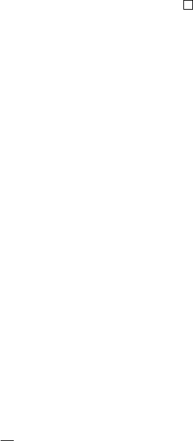
132 the polynomial method proof of roth’s theorem in the finite field model
Therefore α = O(1/ log log N) and |A| = αN = O(N/ log log N), as
desired.
Remark 6.19. This is the same proof in spirit as last time. A theme
in additive combinatorics is that the finite field model is a nice play-
ground for most techniques.
Let us compare this proof strategy in both F
n
3
and [N]. We saw
that r
3
(F
n
3
) = O(N/ log N). However, the bound for [N] is O(N/ log log N),
which is weaker by a log factor. Where does this stem from? Well, in
the density increment step for F
n
3
, we were able to pass down to a
subset which had size a constant factor of the original one. How-
ever, in [N], each iteration gives us a subprogression which has size
equal to the cube root of the previous subspace. This poses a nat-
ural question—is it possible to pass down to subsprogressions of
[N] which look more like subspaces? It turns out that this is indeed
possible.
For a subset S ⊂ F
n
3
, we can write its orthogonal complement as
U
S
= {x ∈ F
n
3
: x ·s = 0 for all s ∈ S}.
In [N], the analogous concept is known as a Bohr set, an idea de-
veloped by Bourgain to transfer the proof in Section 6.1 to Z. This Bourgain, 1999
requires us to work in Z/NZ. For some subset S ⊂ Z/NZ, we can
define its Bohr set as
Bohr(S, e) = {x ∈ Z/NZ :
sx
N
≤ e for all s ∈ S}.
This provides a more natural analogy to subspaces, and is the basis
for modern improvements on bounds to Roth’s Theorem. We will
study Bohr sets in relation to Freiman’s Theorem in Chapter 7.
6.3 The polynomial method proof of Roth’s theorem in the finite
field model
11/20: Swapnil Garg and Alan Peng
Currently, the best known bound for Roth’s Theorem in F
n
3
is the
following:
Theorem 6.20. r
3
(F
n
3
) = O(2.76
n
). Ellenberg and Gijswijt (2017)
This bound improves upon the O(3
n
/n
1+e
) bound (for some
e > 0) proved earlier by Bateman and Katz. Bateman and Katz Bateman and Katz (2012)
used Fourier-analytic methods to prove their bound, and until very
recently, it was open whether the upper bound could be improved to
a power-saving one (one of the form O(c
n
) for c < 3), closer to the
lower bound given by Edel of 2.21
n
. Edel (2004)
Croot–Lev–Pach gave a similar bound for 3-APs over (Z/4Z)
n
,
proving that the maximum size of a set in (Z/4Z)
n
with no 4-APs is
roth’s theorem 133
O(3.61
n
). They used a variant of the polynomial method, and their Croot, Lev, and Pach (2017)
proof was made easier by the fact that there are elements of order
2. Ellenberg and Gijswijt used the Croot–Lev–Pach method, as it is
often referred to in the literature, to prove the bound for F
n
3
.
We will use a formulation that appears on Tao’s blog. Tao (2016)
Let A ⊆ F
n
3
be 3-AP-free (this is sometimes known as a cap set in
the literature). Then we have the identity
δ
0
(x + y + z) =
∑
a∈A
δ
a
(x)δ
a
(y)δ
a
(z) (6.2)
for x, y, z ∈ A, where δ
a
is the Dirac delta function, defined as fol-
lows:
δ
a
(x) :=
1 if x = a,
0 if x 6= a.
Note that (6.2) holds because x + y + z = 0 if and only if z − y =
y − x in F
n
3
, meaning that x, y, z form an arithmetic progression,
which is only possible if x = y = z = a for some a ∈ F
n
3
.
We will show that the left-hand side of (6.2) is “low-rank" and the
right-hand side is “high-rank" in a sense we explain below.
Recall from linear algebra the classical notion of rank: given a
function F : A × A → F, for a field F, we say F is rank 1 if it is
nonzero and can be written in the form F(x, y) = f (x)g(y) for some
functions f , g : A → F. In general, we define rank F to be the min-
imum number of rank 1 functions required to write F as a linear
combination of rank 1 functions. We can view F as a matrix.
How should we define the rank of a function F : A × A × A → F?
We might try to extend the above notion by defining such a function
F to be rank 1 if F(x, y, z) = f (x)g(y)h(z), known as tensor rank, but
this is not quite what we want. Instead, we say that F has slice-rank
1 if it is nonzero and it can be written in one of the forms f (x)g(y, z),
f (y)g(x, z), or f (z)g(x, y). In general, we say the slice-rank of F is
the minimum number of slice-rank 1 functions required to write F
as a linear combination. For higher powers of A, we generalize this
definition accordingly.
What is the rank of a diagonal function? Recall from linear algebra
that the rank of a diagonal matrix is the number of nonzero entries.
A similar result holds true for the slice-rank.
Lemma 6.21. If F : A × A × A → F equals
F(x, y, z) =
∑
a∈A
c
a
δ
a
(x)δ
a
(y)δ
a
(z),
then
slice-rank F = |{a ∈ A : c
a
6= 0}|.

134 the polynomial method proof of roth’s theorem in the finite field model
Here the coefficients c
a
correspond to diagonal entries.
Proof. It is clear that slice-rank F ≤ |{a ∈ A : c
a
6= 0}|, as we can write
F as a sum of slice-rank 1 functions by
F(x, y, z) =
∑
a∈A
c
a
6=0
c
a
δ
a
(x)(δ
a
(y)δ
a
(z)).
For the other direction, assume that all diagonal entries are nonzero;
if c
a
= 0 for some a, then we can remove a from A without increasing
the slice-rank. Now suppose slice-rank F < |A|. So we can write
F(x, y, z) = f
1
(x)g
1
(y, z) + ···+ f
`
(x)g
`
(y, z)
+ f
`+1
(y)g
`+1
(x, z) + ···+ f
m
(y)g
m
(x, z)
+ f
m+1
(z)g
m+1
(x, y) + ···+ f
|A|−1
(z)g
|A|−1
(x, y).
Claim 6.22. There exists h : A → F
3
with |supp h| > m such that
∑
z∈A
h(z) f
i
(z) = 0 (6.3)
for all i = m + 1, . . . , |A| −1.
Here supp h is the set {z ∈ A : h(z) 6= 0}.
Proof. In the vector space of functions A → F
3
, the set of h satisfying
(6.3) for all i = m + 1, . . . , |A| − 1 is a subspace of dimension greater
than m. Furthermore, we claim that every subspace of dimension m +
1 has a vector whose support has size at least m + 1. For a subspace
X of dimension m + 1, suppose we write m + 1 vectors forming a
basis of X in an |A| × (m + 1) matrix Y. Then, this matrix has rank
m + 1, so there must be some non-vanishing minor of order m + 1;
that is, we can delete some rows of Y to get an (m + 1) × (m + 1)
matrix with nonzero determinant. If the column of this matrix are
the vectors v
1
through v
m+1
, then these vectors generate all of F
m+1
3
.
In particular, some linear combination of v
1
, v
2
, . . . , v
m+1
is equal to
the vector of all ones, which has support m + 1. So, taking that linear
combination of the original vectors (the columns of Y) gives a vector
of support at least m + 1.
Pick the h from the claim. We find
∑
z∈A
F(x, y, z)h(z) =
∑
a∈A
∑
z∈A
c
a
δ
a
(x)δ
a
(y)δ
a
(z)h(z) =
∑
a∈A
c
a
h(a)δ
a
(x)δ
a
(y),
but also
∑
z∈A
F(x, y, z)h(z) = f
1
(x)
e
g
1
(y) + ··· + f
`
(x)
]
g
`
(y)
+ f
`+1
(y)
g
g
`+1
(x) + ··· + f
m
(y)
f
g
m
(x),

roth’s theorem 135
where
e
g
i
(y) =
∑
z∈A
g
i
(y, z)h(z) for 1 ≤ i ≤ `, and
e
g
i
(x) =
∑
z∈A
g
i
(x, z)h(z) for ` + 1 ≤ i ≤ m. Thus
∑
a∈A
c
a
h(a)δ
a
(x)δ
a
(y) = f
1
(x)
e
g
1
(y) + ··· + f
`
(x)g
`
(y)
+ f
`+1
(y)
g
g
`+1
(x) + ··· + f
m
(y)
f
g
m
(x).
Note the left-hand side has more than m diagonal entries (namely the
a where h(a) 6= 0), but the left-hand side has rank at most m, which is
a contradiction as we have reduced to the 2-dimensional case.
Using induction, we can easily generalize (from 3 variables) to any
finite number of variables, the proof of which we omit.
We have thus proved that the slice-rank of the right hand side of
(6.2) is |A|, and is therefore “high-rank.” We now show that the left
hand side has “low-rank.”
Lemma 6.23. Define F : A × A × A → F
3
as follows:
F(x + y + z) := δ
0
(x + y + z).
Then slice-rank F ≤ 3M, where
M :=
∑
a,b,c≥0
a+b+c=n
b+2c≤2n/3
n!
a!b!c!
.
Proof. In F
3
, one has δ
0
(x) = 1 − x
2
. Applying this coordinate-wise,
δ
0
(x + y + z) =
n
∏
i=1
(1 − (x
i
+ y
i
+ z
i
)
2
), (6.4)
where the x
i
are the coordinates of x ∈ F
n
3
, and so on. If we expand
the right-hand side, we obtain a polynomial in 3n variables with
degree 2n. We find a sum of monomials, each of the form
x
i
1
1
···x
i
n
n
y
j
1
1
···y
j
n
n
z
k
1
1
···z
k
n
n
,
where i
1
, i
2
, . . . , i
n
, j
1
, . . . , j
n
, k
1
, . . . , k
n
∈ {0, 1, 2}. Group these mono-
mials. For each term, by the pigeonhole principle, at least one of
i
1
+ ··· + i
n
, j
1
+ ··· + j
n
, k
1
+ ··· + k
n
is at most 2n/3.
We can write (6.4) as a sum of monomials, which we write explic-
itly as
n
∏
i=1
(1 −(x
i
+ y
i
+ z
i
)
2
) =
∑
i
1
,i
2
,...,i
n
j
1
,j
2
,...,j
n
k
1
,k
2
,...,k
n
c
i
1
,...,i
n
,j
1
,...,j
n
,k
1
,...,k
n
x
i
1
1
···x
i
n
n
y
j
1
1
···y
j
n
n
z
k
1
1
···z
k
n
n
(6.5)

136 the polynomial method proof of roth’s theorem in the finite field model
where c
i
1
,...,i
n
,j
1
,...,j
n
,k
1
,...,k
n
is a coefficient in F
3
. Then, we can group
terms to write (6.5) as a sum of slice-rank 1 functions in the following
way:
n
∏
i=1
(1 − (x
i
+ y
i
+ z
i
)
2
) =
∑
i
1
+···+i
n
≤
2n
3
x
i
1
1
···x
i
n
n
f
i
1
,...,i
n
(y, z)
+
∑
j
1
+···+j
n
≤
2n
3
y
j
1
1
···y
j
n
n
g
j
1
,...,j
n
(x, z)
+
∑
k
1
+···+k
n
≤
2n
3
z
k
1
1
···z
k
n
n
h
k
1
,...,k
n
(x, y),
where
f
i
1
,...,i
n
(y, z) =
∑
j
1
,j
2
,...,j
n
k
1
,k
2
,...,k
n
c
i
1
,...,i
n
,j
1
,...,j
n
,k
1
,...,k
n
y
j
1
1
···y
j
n
n
z
k
1
1
···z
k
n
n
,
and g
j
1
,...,j
n
(x, z) and h
k
1
,...,k
n
(x, y) are similar except missing some
terms to avoid overcounting.
So, each monomial with degree at most 2n/3 contributes to the
slice-rank 3 times, and the number of such monomials is at most M.
Thus the slice-rank is at most 3M.
We would like to estimate M. If we let 0 ≤ x ≤ 1, we see that
Mx
2n/3
≤ (1 + x + x
2
)
n
if we expand the right-hand side. Explicitly,
Mx
2n/3
≤
∑
a,b,c≥0
a+b+c=n
b+2c≤2n/3
x
b+2c
n!
a!b!c!
≤ (1 + x + x
2
)
n
.
So
M ≤ inf
0<x<1
(1 + x + x
2
)
n
x
2n/3
≤ (2.76)
n
,
where we plug in x = 0.6. Alternatively, we could Stirling’s
formula, which would give the same
bound.
When this proof came out, people were shocked; this was basi-
cally a four-page paper, and demonstrated the power of algebraic
methods. However, these methods seem more fragile compared to
the Fourier-analytic methods we used last time. It is an open prob-
lem to extend this technique to prove a power-saving upper-bound
for the size of a 4-AP-free subset of F
n
5
(in the above arguments, we
can replace F
3
with any other finite field, so the choice of field does
not really matter). It is also open to extend the polynomial method
to corner-free sets in F
n
2
× F
n
2
, where corners are sets of the form
{(x, y), (x + d, y), (x, y + d)}, or to the integers.

roth’s theorem 137
6.4 Roth’s theorem with popular differences
After giving a new method for 3-APs in F
n
3
that gave a much better
bound than Fourier analysis, we will now give a different proof that
gives a much worse bound, but has strong consequences.
This theorem involves a “popular common difference."
Theorem 6.24. For all e > 0, there exists n
0
= n
0
(e) such that for Green (2005)
n ≥ n
0
and every A ⊆ F
n
3
with |A| = α3
n
, there exists y 6= 0 such that
|{x : x, x + y, x + 2y ∈ A}| ≥ (α
3
−e)3
n
.
Here y is the popular common difference; this theorem obtains
a lower bound on the number of 3-APs with common difference y
in A. Note that α
3
3
n
is roughly the expected number of 3-APs with
common difference y if A is a random subset of F
n
3
with size α3
n
. The
theorem states we can find some y such that the number of 3-APs
with common difference y is close to what we expect in a random set,
and suggests that it is not true that the number of 3-APs is at least
what we would expect in a random set.
Green showed that the theorem is true with n
0
= tow((1/e)
O(1)
).
This bound was improved by Fox–Pham to n
0
= tow(O(log
1
e
)),
using the regularity method. They showed that this bound is tight; Fox and Pham (2019+)
this is an instance in which the regularity method gives the right
bounds, which is interesting. This is the bound we will show.
Lemma 6.25 (Bounded increments). Let α, e > 0. If α
0
, α
1
, . . . ∈ [0, 1]
such that α
0
≥ α, then there exists k ≤ dlog
2
1
e
e such that 2α
k
− α
k+1
≥
α
3
−e.
Proof. Otherwise, α
1
≥ 2α
0
− α
3
+ e ≥ α
3
+ e. Similarly α
2
≥ 2α
1
−
α
3
+ e ≥ α
3
+ 2e. If we continue this process, we find α
k
≥ α
3
+ 2
k−1
e
for all 1 ≤ k ≤ dlog
2
1
e
e+1. Thus α
k
> 1 if k = dlog
2
1
e
e + 1, which is a
contradiction.
Let f : F
n
3
→ C, and let U ≤ F
n
3
; this notation means that U is a
subspace of F
n
3
. Let f
U
(x) be the average of f (x) on the U-coset that
x is in.
The lemma below is related to an arithmetic analog of the regular-
ity lemma.
Lemma 6.26. For all e > 0, there exists m = tow(O(log
1
e
)) such that for
all f : F
n
3
→ [0, 1], there exist subspaces W ≤ U ≤ F
n
3
with codim W ≤ m
such that
k
\
f − f
W
k
∞
≤
e
|U
⊥
|
and
2kf
U
k
3
3
−kf
W
k
3
3
≥ (E f )
3
−e.

138 roth’s theorem with popular differences
Proof. Let e
0
:= 1 and e
k+1
:= e3
−1/e
2
k
for integers k ≥ 0. Using the
recursion, we find that the recursion says e
−2
k+1
= e
−2
3
2/e
2
k
, so that
e
−2
k+1
≤ 2
2
e
−2
k
for sufficiently large k. Let
R
k
:= {r ∈ F
n
3
: |
ˆ
f (r)| ≥ e
k
}.
Then |R
k
| ≤ e
−2
k
, since by Parseval’s identity,
∑
r
|
ˆ
f (r)|
2
= E[ f
2
] ≤ 1.
Now define U
k
:= R
⊥
k
and α
k
:= kf
U
k
k
3
3
. Note α
k
≥ ( E f )
3
by
convexity. So by the previous lemma, there exists k = O(log
1
e
) such
that 2α
k
− α
k+1
≥ (E f )
3
− e. For this choice of k, let m := e
−2
k+1
. With
some computation we find m = tow(O( log
1
e
)).
It is not too hard to check that
c
f
W
(r) =
ˆ
f (r) if r ∈ W
⊥
,
0 if r /∈ W
⊥
.
So k
\
f − f
U
k+ 1
k
∞
≤ max
r/∈R
k+ 1
|
ˆ
f (r)| ≤ e
k+1
≤ 3
−|R
k
|
e ≤ e/|U
⊥
k
|. So
if we take W = U
k+1
and U = U
k
, we are done, as codim U
k+1
≤
|R
k+1
| ≤ m.
With a regularity lemma comes a counting lemma, which is left as
an exercise (it is fairly easy to prove). Define
Λ
3
( f ; U) = E
x∈F
n
3
,y∈U
f (x) f (x + y) f (x + 2y).
Lemma 6.27 (Counting lemma). Let f , g : F
n
3
→ [0, 1] and U ≤ F
n
3
.
Then
|Λ
3
( f ; U) − Λ
3
(g; U)| ≤ 3|U
⊥
|· k
[
f − gk
∞
.
Lemma 6.28. Let f : F
n
3
→ [0, 1] , with subspaces W ≤ U ≤ F
n
3
. Then
Λ
3
( f
W
; U) ≥ 2kf
U
k
3
3
−kf
W
k
3
3
.
Proof. We use Schur’s inequality: a
3
+ b
3
+ c
3
+ 3abc ≥ a
2
(b + c) +
b
2
(a + c) + c
2
(a + b) for a, b, c ≥ 0. We find
Λ( f
W
; U) = E
x,y,z
form a 3-AP in
the same U-coset
f
W
(x) f
W
(y) f
W
(z)
≥ 2E
x, y in same U-coset
f
W
(x)
2
f
W
(y) −E f
3
W
≥ 2E f
2
W
f
U
−E f
3
W
≥ 2E f
3
U
−E f
3
W
,
where the first inequality follows from Schur’s inequality and the last
follows from convexity.

roth’s theorem 139
Theorem 6.29. For all e > 0, there exists m = tow(O(log
1
e
)) such that if
f : F
n
3
→ [0, 1], then there exists U ≤ F
n
3
with codimension at most m such
that
Λ
3
( f ; U) ≥ (E f )
3
−e.
Note if n is large enough, then |U| is large enough, so there exists
a nonzero “common difference" y.
Proof. Choose U, W as in the regularity lemma. Then
Λ
3
( f ; U) ≥ Λ
3
( f
W
; U) − 3e ≥ 2kf
U
k
3
3
−kf
W
k
3
3
−3e ≥ (E f )
3
−4e.
The corresponding statement for popular differences is true in Z
as well.
Theorem 6.30. For all e > 0, there exists N
0
= N
0
(e) such that if Green (2005)
N > N
0
and A ⊆ [N] with |A| = αN, then there exists y > 0 such that
|{x : x, x + y, x + 2y ∈ A}| ≥ (α
3
−e)N.
A similar statement also holds for 4-APs in Z:
Theorem 6.31. For all e > 0, there exists N
0
= N
0
(e) such that if Green and Tao (2010)
N > N
0
and A ⊆ [N] with |A| = αN, then there exists y > 0 such that
|{x : x, x + y, x + 2y, x + 3y ∈ A}| ≥ (α
4
−e)N.
Remark 6.32. Surprisingly, the corresponding statement for 5-APs (or
longer) in Z is false. Bergelson, Host, and Kra (2005) with
appendix by Ruzsa

7
Structure of set addition
7.1 Structure of sets with small doubling
11/25: Adam Ardeishar
One of the main goals of additive combinatorics can be roughly de-
scribed as understanding the behavior of sets under addition. In
order to discuss this more precisely, we will begin with a few defini-
tions.
Definition 7.1. Let A and B be finite subsets of an abelian group.
Their sumset is defined as A + B = {a + b|a ∈ A, b ∈ B}. We can fur-
ther define A − B = {a − b|a ∈ A, b ∈ B} and kA = A + A + ··· + A
| {z }
k times
where k is a positive integer. Note that this is different from mul-
tiplying every element in A by k, which we denote the dilation
k · A = {kA|a ∈ A}.
Given a finite set of integers A, we want to understand how its
size changes under these operations, giving rise to the following
natural question:
Question 7.2. How large or small can |A + A| be for a given value of
|A| where A ⊂ Z?
It turns out that this is not a hard question. In Z, we have precise
bounds on the size of the sumset given the size of the set.
Proposition 7.3. If A is a finite subset of Z, then
2|A| −1 ≤ |A + A| ≤
|A| + 1
2
.
Proof. The right inequality follows from the fact that there are only
(
|A|+1
2
)
unordered pairs of elements of A.
If the elements of A are a
1
< a
2
< ··· < a
|A|
, then note that
a
1
+ a
1
< a
1
+ a
2
< ··· < a
1
+ a
|A|
< a
2
+ a
|A|
< ··· < a
|A|
+ a
|A|
is an increasing sequence of 2|A| − 1 elements of |A + A|, so the left
inequality follows.

142 structure of sets with small doubling
The upper bound is tight when there are no nontrivial collisions in
A + A, that is, there are no nontrivial solutions to a
1
+ a
2
= a
0
1
+ a
0
2
for a
1
, a
2
, a
0
1
, a
0
2
∈ A.
Example 7.4. If A = {1, a, a
2
, . . . , a
n−1
} ⊂ Z for a > 1, then |A + A| =
(
n+1
2
)
.
The lower bound is tight when A is an arithmetic progression.
Even if we instead consider arbitrary abelian groups, the problem is
similarly easy. In a general abelian group G, we only have the trivial
inequality |A + A| ≥ |A|, and equality holds if A is a coset of some
finite subgroup of G. The reason we have a stronger bound in Z is
that there are no nontrivial finite subgroups of Z.
A more interesting question that we can ask is what can we say
about sets where |A + A| is small. More precisely:
Definition 7.5. The doubling constant of a finite subset A of an
abelian group is the ratio |A + A|/|A|.
Question 7.6. What is the structure of a set with bounded doubling
constant (e.g. |A + A| ≤ 100|A|)?
We’ve already seen an example of such a set in Z, namely arith-
metic progressions.
Example 7.7. If A ⊂ Z is a finite arithmetic progression, |A + A| =
2|A| −1 ≤ 2|A|, so it has doubling constant at most 2.
Moreover if we delete some elements of an arithmetic progression,
it should still have small doubling. In fact, if we delete even most
of the elements of an arithmetic progression but leave a constant
fraction of the progression remaining, we will have small doubling.
Example 7.8. If B is a finite arithmetic progression and A ⊆ B has
|A| ≥ C|B|, then |A + A| ≤ |B + B| ≤ 2|B| ≤ 2C
−1
|A|, so A has
doubling constant at most 2/C.
A more substantial generalization of this is a d-dimensional arith-
metic progression.
Figure 7.1: Picture of a 2-dimensional
arithmetic progression as a projection of
a lattice in Z
2
into Z.
Definition 7.9. A generalized arithmetic progression (GAP) of di-
mension d is a set of the form
{x
0
+ `
1
x
1
+ ··· + `
d
x
d
| 0 ≤ `
1
< L
d
, . . . , 0 ≤ `
d
< L
d
, `
1
, . . . , `
d
∈ Z}
where x
0
, x
1
, . . . , x
d
∈ Z and L
1
, . . . , L
d
∈ N. The size of a GAP is
defined as L
1
L
2
···L
d
. If there are no nontrivial coincidences among
the elements of the GAP, it is called proper.
Remark 7.10. Note that if a GAP is not proper, the size is not equal to
the number of distinct elements, i.e. its cardinality.

structure of set addition 143
It is not too hard to see that a proper GAP of dimension d has
doubling constant at most 2
d
. Furthermore, we have the same prop-
erty that deleting a constant fraction of the elements of a GAP will
still leave a set of small doubling constant. We have enumerated sev-
eral examples of sets of small doubling constant, so it is natural to
ask whether we can give an exact classification of such sets. We have
an “inverse problem” to Question 7.6, asking whether every set with
bounded doubling constant must be one of these examples.
This is not such an easy problem. Fortunately, a central result in
additive combinatorics gives us a positive answer to this question.
Theorem 7.11 (Freiman’s theorem). If A ⊂ Z is a finite set and |A + Freiman (1973)
A| ≤ K|A|, then A is contained in a GAP of dimension at most d(K) and
size at most f (K)|A|, where d(K) and f (K) are constants depending only
on K.
Remark 7.12. The conclusion of the theorem can be made to force the
GAP to be proper, at the cost of increasing d(K) and f (K), using the
fact below, whose proof we omit but can be found as Theorem 3.40 in
the textbook by Tao and Vu. Tao and Vu (2006)
Theorem 7.13. If P is a GAP of dimension d, then P is contained in a
proper GAP Q of dimension at most d and size at most d
C
0
d
3
|P| for some
absolute constant C
0
> 0.
Freiman’s theorem gives us significant insight into the structure of
sets of small doubling. We will see the proof of Freiman’s theorem in
the course of this chapter. Its proof combines ideas from Fourier anal-
ysis, the geometry of numbers, and classical additive combinatorics.
Freiman’s original proof was difficult to read and did not origi-
nally get the recognition it deserved. Later on Ruzsa found a simpler
proof, whose presentation we will mostly folllow. The theorem is Ruzsa (1994)
sometimes called the Freiman–Ruzsa theorem. Freiman’s theorem
was brought into prominence as it and its ideas play central roles in
Gowers’ new proof of Szemerédi’s theorem.
If we consider again Example 7.4, then we have K =
|A|+1
2
=
Θ(|A|). There isn’t really a good way to embed this into a GAP. If we
let the elements of A be a
1
< a
2
< ··· < a
|A|
, we can see that it is
contained in a GAP of dimension |A| − 1 and size 2
|A|−1
, by simply
letting x
0
= a
1
, x
i
= a
i+1
− a
1
, and L
i
= 2 for 1 ≤ i ≤ |A| − 1.
Then this indicates that the best result we can hope for is showing
d(K) = O( K) and f (K) = 2
O(K)
. This problem is still open.
Open problem 7.14. Is Theorem 7.11 true with d(K) = O(K) and
f (K) = 2
O(K)
?
The best known result is due to Sanders, who also has the best
known bound for Roth’s Theorem (Theorem 6.12).
144 plünnecke–ruzsa inequality
Theorem 7.15 (Sanders). Theorem 7.11 is true with d(K) = K(log K)
O(1)
, Sanders (2012)
In the asymptotic notation we assume
that K is sufficiently large, say K ≥ 3, so
that log K is not too small.
f (K) = e
K(log K)
O(1)
.
Similar to how we discussed Roth’s theorem, we will begin by
analyzing a finite field model of the problem. In F
n
2
, if |A + A| ≤
K|A|, then what would A look like? If A is a subspace, then it has
doubling constant 1. A natural analogue of our inverse problem is to
ask if all such A are contained in a subspace that is not much larger
than A.
Theorem 7.16 (F
n
2
-analogue of Freiman). If A ⊂ F
n
2
has |A + A| ≤
K|A|, then A is contained in a subspace of cardinality at most f (K)|A|,
where f (K) is a constant depending only on K.
Remark 7.17. If we let A be a linearly independent set (i.e. a basis),
then K = Θ(|A|) and the smallest subspace containing A will have
cardinality 2
|A|
. Thus f (K) must be exponential in K at least. We’ll
prove Theorem 7.16 in Section 7.3.
7.2 Plünnecke–Ruzsa inequality
Before we can prove Freiman’s theorem (Theorem 7.11) or its finite
field version (Theorem 7.16), we will need a few tools. We begin with
one of many results named after Ruzsa.
Theorem 7.18 (Ruzsa triangle inequality). If A, B, C are finite subsets of
an abelian group, then
|A||B −C| ≤ |A − B||A −C|.
Proof. We will construct an injection
φ : A ×(B −C) ,→ (A − B) × (A −C).
For each d ∈ B − C, we can choose b(d) ∈ B, c(d) ∈ C such that
d = b(d) − c(d). Then define φ(a, d) = (a − b(d), a − c(d)). This is
injective because if φ(a, d) = (x, y), then we can recover (a, d) from
(x, y) because d = y −x and a = x + b(y − x).
Remark 7.19. By replacing B with −B and/or C with −C, we can
change some of the plus signs into minus signs in this inequality. Un-
fortunately, this trick cannot be used to prove the similar inequality
|A||B + C| ≤ |A + B||A + C|. Nevertheless, we will soon see that this
inequality is still true.
Remark 7.20. Where’s the triangle? If we define ρ(A, B) = log
|A−B|
√
|A||B|
,
then Theorem 7.18 states that ρ(B, C) ≤ ρ(A, B) + ρ(A, C). This
looks like the triangle inequality, but unfortunately ρ is not actually a
metric because ρ(A, A) 6= 0 in general. If we restrict to only looking
at subgroups, however, then ρ is a bona fide metric.

structure of set addition 145
The way that we use Theorem 7.18 is to control further doublings
of a set of small doubling. Its usefulness is demonstrated by the
following example.
Example 7.21. Suppose A is a finite subset of an abelian group with
|2A −2A| ≤ K|A|. If we set B = C = 2A − A in Theorem 7.18, then
we get
|3A −3A| ≤
|2A −2A|
2
|A|
≤ K
2
|A|.
We can repeat this with B = C = 3A −2A to get
|5A −5A| ≤
|3A −3A|
2
|A|
≤ K
4
|A|
and so on, so for all m we have that |mA − mA| is bounded by a
constant multiple of |A|.
The condition |2A − 2A| ≤ K|A| is stronger than the condition
|A + A| ≤ K|A|. If we want to bound iterated doublings given just
the condition |A + A| ≤ K|A|, we need the following theorem.
Theorem 7.22 (Plünnecke–Ruzsa inequality). If A is a finite subset of Plünnecke (1970)
Ruzsa (1989)
We think of polynomial changes in K as
essentially irrelevant, so this theorem
just says that if a set has small doubling
then any iteration of the set is also
small.
an abelian group and |A + A| ≤ K|A|, then |mA −nA| ≤ K
m+n
|A|.
Remark 7.23. Plünnecke’s original proof of the theorem did not re-
ceive much attention. Ruzsa later gave a simpler proof of Plünnecke’s
theorem. Their proofs involved the study of an object called a com-
mutative layered graph, and involved Menger’s theorem for flows
and the tensor power trick. Recently Petridis gave a significantly sim- Petridis (2012)
pler proof which uses some of the earlier ideas, which we will show
here.
In proving this theorem, we will generalize to the following theo-
rem.
Set B = A to recover Theorem 7.22
Theorem 7.24. If A and B are finite subsets of an abelian group and |A +
B| ≤ K|A|, then |mB − nB| ≤ K
m+n
|A|.
Petridis’ proof relies on the following key lemma.
Lemma 7.25. Suppose A and B are finite subsets of an abelian group. If
X ⊆ A is a nonempty subset which minimizes
|X+B|
|X|
, and K
0
=
|X+B|
|X|
, then
|X + B + C| ≤ K
0
|X + C| for all finite sets C.
Remark 7.26. We can think of this lemma in terms of a bipartite
graph. If we consider the bipartite graph on vertex set G
1
t G
2
, where
G
1
, G
2
are copies of the ambient abelian group G, with edges from g
to g + b for any g ∈ G
1
, g + b ∈ G
2
where b ∈ B. Then if N(S) denotes
the neighborhood of a set of vertices S, then the lemma is considering
146 plünnecke–ruzsa inequality
the expansion ratio
|N(A)|
|A|
=
|A+B|
|A|
. The lemma states that if X is a set
whose expansion ratio K
0
is less than or equal to the expansion ratio
of any of its subsets, then for any set C, X + C also has expansion
ratio at most K
0
.
G G
+B
A
A + B
Figure 7.2: Bipartite graph where edges
correspond to addition by an element of
B.
Proof of Theorem 7.24 assuming Lemma 7.25. Assuming the key lemma,
let us prove the theorem. Let X be a nonempty subset of A minimiz-
ing
|X+B|
|X|
, and let K
0
=
|X+B|
|X|
. Note that K
0
≤ K by minimality. Ap-
plying the lemma with C = rB where r ≥ 1, we have |X + (r + 1)B| ≤
K
0
|X + rB| ≤ K|X + rB|, so by induction |X + rB| ≤ K
r
|X| for all
r ≥ 0. Applying Theorem 7.18 we have |mB − nB| ≤
|X+mB||X+nB|
|X|
≤
K
m+n
|X| ≤ K
m+n
|A|.
Proof of Lemma 7.25. We will proceed by induction on |C|. The base
case of |C| = 1 is clear because for any finite set S, S + C is a trans-
lation of S so |S + C| = |S|, thus |X + B + C| = |X + B| = K
0
|X| =
K
0
|X + C|.
For the inductive step, assume |C| > 1, let γ ∈ C and C
0
= C\{γ}.
Then
X + B + C = (X + B + C
0
) ∪
(X + B + γ)\(Z + B + γ)
where
Z = {x ∈ X|x + B + γ ⊆ X + B + C
0
}.
Z ⊆ X so by minimality |Z + B| ≥ K
0
|Z|. We have
|X + B + C| ≤ |X + B + C
0
|+ |(X + B + γ)\(Z + B + γ)|
= |X + B + C
0
|+ |X + B|− |Z + B|
≤ K
0
|X + C
0
|+ K
0
|X|− K
0
|Z|
= K
0
(|X + C
0
|+ |X| − |Z|).
Now we want to understand the right hand side X + C. Note that
X + C = (X + C
0
) t
(X + γ)\(W + γ)
where
W = {x ∈ X|x + γ ∈ X + C
0
}.
In particular this is a disjoint union, so
|X + C| = |X + C
0
|+ |X| − |W|.
We also have W ⊆ Z because x + γ ∈ X + C
0
implies x + B + γ ⊆
X + B + C
0
. Thus |W| ≤ |Z|, so
|X + C| ≥ |X + C
0
|+ |X| − |Z|,
which, when combined with the above inequality, completes the
induction.

structure of set addition 147
The key lemma also allows us to replace all the minus signs by
pluses in Theorem 7.18 as promised.
Corollary 7.27. If A, B, C are finite subsets of an abelian group, then
|A||B + C| ≤ |A + B||A + C|.
Proof. Let X ⊆ A be nonempty such that
|X+B|
|X|
is minimal. Let
K =
|A+B|
|A|
, K
0
=
|X+B|
|X|
≤ K. Then
|B + C| ≤ |X + B + C|
≤ K
0
|X + C| (Lemma 7.25)
≤ K
0
|A + C|
≤ K|A + C|
=
|A + B||A + C|
|A|
7.3 Freiman’s theorem over finite fields
11/27: Ahmed Zawad Chowdhury
We have one final lemma to establish before we can prove the finite
field analogue of Frieman’s theorem (Theorem 7.16).
Theorem 7.28 (Ruzsa covering lemma). Let X and B be subsets of an Ruzsa (1999)
In essence, this theorem says that if
it looks like X + B is coverable by K
translates of the set B (based off only
size data), then X is in fact coverable
by K translates of the slightly larger set
B −B.
abelian group. If
|
X + B
|
≤ K
|
B
|
, then there exists a subset T ⊂ X with
|
T
|
≤ K such that X ⊂ T + B −B.
Figure 7.3: A maximal packing of a
region with half balls
Figure 7.4: The maximal packing leads
to a proper covering
The covering analogy provides the intuition for our proof. We
treat the covering sets as balls in a metric space. Now, if we have a
maximal packing of half-sized balls, expanding each to become a unit
ball should produce a covering of the region. Note that maximal here
means no more balls can be placed, not that the maximum possible
number of balls have been placed. We formalize this to prove the
Ruzsa covering lemma.
Proof. Let T ⊂ X be a maximal subset such that t + B is disjoint for
all t ∈ T. Therefore,
|
T
||
B
|
=
|
T + B
|
≤
|
X + B
|
≤ K
|
B
|
. So,
|
T
|
≤ K.
Now, as T is maximal, for all x ∈ X there exists some t ∈ T such
that (t + B) ∩ (x + B) 6= ∅. In other words, there exists b, b
0
∈ B such
that t + b = x + b
0
. Hence x ∈ t + B − B for some t ∈ T. Since this
applies to all x ∈ X, we have X ⊂ T + B − B.
The Ruzsa covering lemma is our final tool required for the proof
of Freiman’s theorem over finite fields (Theorem 7.16). The finite
field model is simpler than working over Z, and so it can be done
with fewer tools compared to the original Freiman’s theorem (Theo-
rem 7.11).

148 freiman’s theorem over finite fields
Now, we will prove Freiman’s theorem in groups with bounded
exponent. This setting is slightly more general than finite fields.
Definition 7.29. The exponent of an abelian group (written addi-
tively) is the smallest positive integer r (if it exists) such that rx = 0
for all elements x of the group.
We also use
h
A
i
to refer to the subgroup of a group G generated
by some subset A of G. By this notation, the exponent of a group
G is max
x∈G
|h
x
i|
. With that notation, we can finally prove Ruzsa’s
analogue of Freiman’s theorem over finite exponent abelian groups.
Theorem 7.30 (Ruzsa). Let A be a finite set in an abelian group with Ruzsa (1999)
This theorem is, in a sense, the converse
of our earlier observation that if A is a
large enough subset of some subgroup
H, then A has small doubling
exponent r < ∞. If
|
A + A
|
≤ K
|
A
|
, then
|h
A
i|
≤ K
2
r
K
4
|
A
|
.
Proof. By the Plünnecke–Ruzsa inequality (Theorem 7.22), we have
|
A + (2A − A)
|
=
|
3A − A
|
≤ K
4
|
A
|
.
Now, from the Ruzsa Covering Lemma (with X = 2A − A, B = A),
there exists some T ⊂ 2A − A with
|
T
|
≤ K
4
such that
2A − A ⊂ T + A − A.
Adding A to both sides, we have,
3A − A ⊂ T + 2A − A ⊂ 2T + A − A.
Iterating this, we have for any positive integer n,
(n + 1)A − A ⊂ nT + A − A ⊂
h
T
i
+ A − A.
Using the Ruzsa Covering Lemma
allowed us to control the expression
nA − A nicely. If we had only used
the Plünnecke–Ruzsa inequality (The-
orem 7.22), the argument would have
failed as the exponent of K would’ve
blown up.
For sufficiently large n, we have nA =
h
A
i
. Thus we can say,
h
A
i
⊂
h
T
i
+ A − A.
Due to the bounded exponent, we have,
|h
T
i|
≤ r
|
T
|
≤ r
K
4
.
And by the Plünnecke–Ruzsa inequality (Theorem 7.22),
|
A − A
|
≤ K
2
|
A
|
.
Thus we have,
|h
A
i|
≤ r
K
4
K
2
|
A
|
.
structure of set addition 149
Example 7.31. In F
n
2
, if A is an independent subset (e.g. the basis
of some subgroup), then A has doubling constant K ≈
|
A
|
/2, and
|h
A
i|
= 2
|
A
|
≈ 2
2K
|A|. Thus the bound on
|h
A
i|
must be at least
exponential in K.
It has recently been determined very precisely the maximum Even-Zohar (2012)
possible value of
|h
A
i|
/
|
A
|
over all A ⊂ F
∞
2
with
|
A + A
|
/
|
A
|
≤ K.
Asymptotically, it is Θ
2
2K
/K
.
For general r, we expect a similar phenomenon to happen. Ruzsa
conjectured that
|h
A
i|
≤ r
CK
|
A
|
. This result is proven for some r Ruzsa (1999)
such as the primes. Even-Zohar and Lovett (2014)
Our proof for Freiman’s theorem over abelian groups of finite
exponent (Theorem 7.30) does not generalize to the integers. Indeed,
in our proof above,
|h
T
i|
if we were working in Z. The workaround
is to model subsets of Z inside a finite group in a way that partially
preserves additive structure.
7.4 Freiman homomorphisms
To understand any object, you should understand maps between
them and the properties preserved by those maps. This is one of the
fundamental principles of mathematics. For example, when studying
groups we are not concerned with what the labels of the elements
are, but the the relations between them according to the group op-
eration. With manifolds, we do not focus on embeddings in space
but instead maps (e.g. diffeomorphisms) which preserve various
fundamental properties.
In additive combinatorics, our object of study is set addition. So
we must understand maps between sets which preserve, or at least
partially preserve, additive structure. Such maps are referred to as
Freiman homomorphisms.
Definition 7.32. Let A, B be subsets in (possibly different) abelian
groups. We say that φ : A → B is a Freiman s-homomorphism (or a
Freiman homomorphism of order s), if Freiman s-homomorphism partially
remembers additive structure, up to
s-fold sums.
φ(a
1
) + ··· + φ(a
s
) = φ(a
0
1
) + ··· + φ(a
0
s
)
whenever a
1
, . . . , a
s
, a
0
1
, . . . , a
0
s
∈ A satisfy
a
1
+ ··· + a
s
= a
0
1
+ ··· + a
0
s
.
Definition 7.33. If φ : A → B is a bijection, and both φ and φ
−1
are Freiman s-homomorphisms, then φ is said to be a Freiman s-
isomorphism.
Let us look at some examples:

150 modeling lemma
Example 7.34. Every group homomorphism is a Freiman homomor-
phism for any order.
Example 7.35. If φ
1
and φ
2
are both Freiman s-homomorphisms, then
their composition φ
1
◦ φ
2
is also a Freiman s-homomorphism. And if
φ
1
and φ
2
are both Freiman s-isomorphisms, then their composition
φ
1
◦φ
2
is a Freiman s-isomorphism.
Example 7.36. Suppose S has no additive structure (e.g. {1, 10, 10
2
, 10
3
}).
Then an arbitrary map φ : S → Z is a Freiman 2-homomorphism.
Example 7.37. Suppose S
1
and S
2
are both sets without additive
structure. Then any bijection φ : S
1
→ S
2
is a Freiman 2-isomorphism.
Note that Freiman isomorphism and group homomorphisms have
subtle differences!
Example 7.38. The natural embedding φ : {0, 1}
n
→ (Z/2Z)
n
is a
group homomorphism, so it is a Freiman homomorphism of every
order. It is also a bijection. But its inverse map does not preserve
some additive relations, thus it is not a Freiman 2-isomorphism!
In general, the mod N map Z → Z/NZ is a group homomor-
phism, but not a Freiman isomorphism. This holds even if we restrict
the map to [N] rather than Z. However, we can find Freiman isomor-
phisms by restricting to subsets of small diameter.
Proposition 7.39. If A ⊂ Z has diameter smaller than N/s, then (mod N)
maps A Freiman s-isomorphically to its image. If A is restricted to a small interval,
then it does not have its additive
relations wrap around mod N. Thus it
becomes a Freiman isomorphism.
Proof. If a
1
, . . . , a
s
, a
0
1
, . . . , a
0
s
∈ A are such that
s
∑
i=1
a
i
−
s
∑
i=1
a
0
i
≡ 0 (mod N),
then the left hand side, viewed as an integer, has absolute value
less than N (since |a
i
− a
0
i
| < N/s for each i). Thus the left hand
side must be 0 in Z. So the inverse of the mod N map is a Freiman s-
homomorphism over A, and thus mod N is a Freiman s-isomorphism.
7.5 Modeling lemma
When trying to prove Freiman’s theorem over the integers, our main
difficulty is that a subset A with small doubling might be spread out
over Z. But we can use a Freiman isomorphism to model A inside a
smaller space, preserving relative additive stucture. In this smaller
space, we have better tools such as Fourier Analysis. To set up this
model, we prove a modeling lemma. To warm up, let us prove this in
the finite field model.

structure of set addition 151
Theorem 7.40 (Modeling lemma in finite field model). Let A ⊂ F
n
2
with 2
m
≥
|
sA −sA
|
for some positive integer m. Then A is Freiman
s-isomorphic to some subset of F
m
2
. F
n
2
could potentially be very large. But
we can model the additive structure
of A entirely within F
m
2
, which has
bounded size.
Remark 7.41. If |A + A| ≤ K|A|, then by the Plünnecke–Ruzsa in-
equality (Theorem 7.22) we have
|
sA −sA
|
≤ K
2s
|
A
|
, so the hy-
pothesis if the theorem would be satisfied for some m = O(s log K +
log
|
A
|
).
Proof. The following are equivalent for linear maps φ : F
n
2
→ F
m
2
:
1. φ is Freiman s-isomorphic when restricted to A.
2. φ is injective on sA.
3. φ (x) 6= 0 for all nonzero x ∈ sA −sA.
Then let φ : F
n
2
→ F
m
2
be the uniform random linear map. Each
x ∈ sA − sA violates condition (3) with probability 2
−m
. Thus if
2
m
≥
|
sA −sA
|
, then the probability that condition (3) is satisfied is
nonzero. This implies the existence of a Freiman s-isomorphism.
This proof does not work directly in Z as you cannot just choose
a random linear maps. In fact, the model lemma over Z shows that,
in fact, if A ⊂ Z has small doubling, then a large fraction of A can be
modeled inside a small cyclic group whose size is comparable to
|
A
|
.
It turns out to be enough to model a large subset of A, and we will
use the Ruzsa covering lemma later on to recover the structure of the
entire set A.
Theorem 7.42 (Ruzsa modeling lemma). Let A ⊂ Z, s ≥ 2, and N be Ruzsa (1992)
a positive integer such that N ≥
|
sA −sA
|
. Then there exists A
0
⊂ A with
|
A
0
|
≥
|
A
|
/s such that A
0
is Freiman s-isomorphic to a subset of Z/NZ.
Proof. Let q > max(sA − sA) be a prime. For every choice of λ ∈ We just want to take q large enough
to not have to worry about any pesky
details. Its actual size does not really
matter.
[q −1], we define φ as the composition of functions as follows,
φ : Z → Z/qZ
×λ
−→ Z/qZ → [q].
Any unspecified maps refer to the natural embeddings to and from
mod q. The first two maps are group homomorphisms, so they must
be Freiman s-homomorphisms. The last map is not a group homo-
morphism over the whole domain, but it is over small intervals. In
fact, by the pigeonhole principle, for all λ there exists an interval
I
λ
⊂ [q] of length less than q/s such that A
λ
= {a ∈ A : φ(a) ∈ I
λ
}
has more than
|
A
|
/s elements. Thus φ, when restricted to A
λ
, is a
Freiman s-homomorphism.
Now, we take this map and send it to a cyclic group, while pre-
serving Freiman s-homomorphism. We define,
ψ : Z
φ
−→ [q] → Z/NZ.

152 modeling lemma
Claim 7.43. If ψ does not map A
λ
Freiman s-isomorphically to its
image, then there exists some nonzero d = d
λ
∈ sA − sA such that
φ(d) ≡ 0 (mod N).
Proof. Suppose ψ does not map A
λ
Freiman isomorphically to its
image. Thus, there exists a
1
, . . . , a
s
, a
0
1
, . . . , a
0
s
∈ A
λ
such that
a
1
+ ··· + a
s
6= a
0
1
+ ··· + a
0
s
,
but
φ(a
1
) + ··· + φ(a
s
) ≡ φ(a
0
1
) + ··· + φ(a
0
s
) (mod N).
Since φ(A
λ
) ⊂ I
λ
, which is an interval of length less than q/s, we
have,
φ(a
1
) + ··· + φ(a
s
) − φ(a
0
1
) − ··· − φ(a
0
s
)
∈ (−q, q).
By swapping (a
1
, . . . , a
s
) with (a
0
1
, . . . , a
0
s
) if necessary, we assume that
the LHS above is nonnegative, i.e., lies in the interval [0, q).
We set d = a
1
+ ··· + a
s
− a
0
1
− ··· − a
0
s
. Thus d ∈ (sA − sA) \ {0}.
Now, as all the functions composed to form φ are group homomor-
phisms mod q, we have
φ(d) ≡ φ(a
1
) + ··· + φ(a
s
) − φ(a
0
1
) − ··· − φ(a
0
s
) (mod q),
and φ (d) lies in [0, q) by the definition of φ. Thus the two expressions
above are equal. As a result,
φ(d) ≡ 0 (mod N).
Now, for each d ∈ (sA − sA)\{0}, the number of λ such that
φ(d) ≡ 0 (mod N) equals the number of elements of [q −1] divisible
by N. This number is at most (q −1)/N. Note that we are fixing d, but φ is
determined by λ.
Therefore, the total number of λ such that there exists d ∈ (sA −
sA)\{0} with φ(d) ≡ 0 (mod N) is at most
(
|sA − sA| −1
)
(q −
1)/N < q −1. So there exists some λ such that ψ maps A
λ
Freiman
s-isomorphically onto its image. Taking A
0
= A
λ
, our proof is com-
plete.
By summing up everything we know so far, we establish a result
that will help us in the proof of Freiman’s theorem.
Corollary 7.44. If A ⊂ Z with
|
A + A
|
≤ K
|
A
|
, then there exists a
prime N ≤ 2K
16
|
A
|
and some A
0
⊂ A with
|
A
0
|
≥
|
A
|
/8 such that A
0
is
Freiman 8-isomorphic to a subset of Z/NZ.
Proof. By the Plünnecke–Ruzsa inequality (Theorem 7.22),
|
8A −8A
|
≤
K
16
|
A
|
. We choose a prime K
16
≤ N < 2K
16
by Bertrand’s postulate.
Then we apply the modeling lemma with s = 8 and N ≥
|
8A −8A
|
.
Thus there exists a subset A
0
⊂ A with
|
A
0
|
≥
|
A
|
/8 which is
Freiman 8-isomorphic to a subset of Z/NZ.

structure of set addition 153
7.6 Bogolyubov’s lemma
12/2: Allen Liu
In the Ruzsa modeling lemma (Theorem 7.42) we proved that for any
set A of integers with small doubling constant, a large fraction of A
is Freiman isomorphic to a subset of Z/NZ with N not much larger
than the size of A. To prove Freiman’s Theorem, we need to prove
that we can cover A with GAPs. This leads to the natural question of
how to cover large subsets of Z/NZ with GAPs. In this section, we
first show how to find additive structure within subsets of Z/NZ.
Later on, we will show how to use this additive structure to obtain a
covering. It will be easier to first consider the analogous question in
the finite field F
n
2
. Note a subset of F
n
2
of size α2
n
does not necessar-
ily contain any large structure such as a subspace. However, the key
intuition for this section is the following: given a set A, the sumset
A + A smooths out the structure of A. With this intuition, we arrive
at the following natural question:
Question 7.45. Suppose A ⊂ F
n
2
and |A| = α2
n
where α is a constant
independent of n. Must it be the case that A + A contains a large
subspace of codimension O
α
(1)?
The answer to the above question is no, as evidenced by the fol-
lowing example.
Example 7.46. Let A
n
be the set of all points in F
n
2
with hamming
weight (number of 1 entries) at most (n − c
√
n)/2. Note by the cen-
tral limit theorem
|A
n
| ∼ k2
n
where k > 0 is a constant depending only on c. However, A
n
+ A
n
consists of points in the boolean cube whose Hamming weight is at
most n −c
√
n and thus does not contain any subspace of dimension
> n − c
√
n. The proof of this claim is left as an exercise to the reader.
(The same fact was also used in the proof of (6.3).)
Returning to the key intuition that the sumset A + A smooths out
the structure of A, it is natural to consider sums of more copies of A.
It turns out that if we replace A + A with 2A −2A in Question 7.45
then the answer is affirmative.
Theorem 7.47 (Bogolyubov’s lemma). If A ⊂ F
n
2
and |A| = α2
n
Bogolyubov (1939)
where α is a constant independent of n then 2A −2A contains a subspace of
codimension at most 1/α
2
.
Proof. Let f = 1
A
∗ 1
A
∗ 1
−A
∗ 1
−A
. Note that f is supported on
2A −2A. Next, by the convolution property in Proposition 6.4,
b
f =
b
1
2
A
b
1
2
−A
= |
b
1
A
|
4
.

154 bogolyubov’s lemma
By Fourier inversion, we have
f (x) =
∑
r∈F
n
2
b
f (r)(−1)
r·x
=
∑
r∈F
n
2
|
b
1
A
(r)|
4
(−1)
r·x
.
Note that it suffices to find a subspace where f is positive since
f (x) > 0 would imply x ∈ 2A −2A. We will choose this subspace by
looking at the size of the Fourier coefficients. Let
R = {r ∈ F
n
2
\{0} : |
b
1
A
(r)| > α
3/2
}.
By Parseval’s identity, |R| < 1/α
2
. Next note
∑
r/∈R∪{0}
|
b
1
A
(r)|
4
≤ α
3
∑
r/∈R∪{0}
|
b
1
A
(r)|
2
< α
4
.
If x is in R
⊥
, the orthogonal complement of R, then
f (x) =
∑
r∈F
n
2
|
b
1
A
(r)|
4
(−1)
r·x
≥ |
b
1
A
(0)|
4
+
∑
r∈R
|
b
1
A
(r)|
4
(−1)
r·x
−
∑
r/∈R∪{0}
|
b
1
A
(r)|
4
> α
4
+
∑
r∈R
|
b
1
A
(r)|
4
−α
4
≥ 0.
Thus R
⊥
⊂ supp( f ) = 2A −2A and since |R| < 1/α
2
, we have found
a subspace with the desired codimension contained in 2A −2A.
Our goal is now to formulate an analogous result for a cyclic
group Z/NZ. The first step is to formulate an analog of subspaces
for the cyclic group Z/NZ. Note we encountered a similar issue in
transferring the proof of Roth’s theorem from finite fields to the inte-
gers (see Theorem 6.2 and Theorem 6.12). It turns out that the correct
analog is given by a Bohr set. Recall the definition of a Bohr set:
Definition 7.48. Suppose R ⊂ Z/NZ. Define
Bohr(R, e) = {x ∈ Z/NZ :
rx
N
≤ e, for all r ∈ R}
where
k
·
k
denotes the distance to the nearest integer. We call |R| the
dimension of the Bohr set and e the width.
It turns out that Bogolyubov’s lemma holds over Z/NZ after re-
placing subspaces by Bohr sets of the appropriate dimension. Note
that the dimension of a Bohr set of Z/NZ corresponds to the codi-
mension of a subspace of F
n
2
.
Theorem 7.49 (Bogolyubov’s lemma in Z/NZ). If A ⊂ Z/NZ Bogolyubov (1939)
and |A| = αN then 2A −2A contains some Bohr set Bohr(R, 1/4) with
|R| < 1/α
2
.

structure of set addition 155
Recall the definition of the Fourier Transform over Z/NZ.
Definition 7.50. Fourier transform of f : Z/NZ → C is the function
ˆ
f : Z/NZ → C given by
b
f (r) = E
x∈Z/NZ
f (x)ω
−rx
where ω = e
(2πi)/N
.
We leave it as an exercise to the reader to verify the Fourier inver-
sion formula, Parseval’s identity, Plancherel’s identity and the other
basic properties of the Fourier transform. Now we will prove The-
orem 7.49. It follows the same outline as the proof of Theorem 7.47
except for a few minor details.
Proof of Theorem 7.49. Let f = 1
A
∗1
A
∗1
−A
∗1
−A
. Note that f is sup-
ported on 2A −2A. Next, by the convolution property in Proposition
Proposition 6.4,
b
f =
b
1
2
A
b
1
2
−A
= |
b
1
A
|
4
.
By Fourier inversion, we have
f (x) =
∑
r∈Z/NZ
b
f (r)ω
rx
=
∑
r∈Z/NZ
|
b
1
A
(r)|
4
cos
2πrx
N
.
Let
R = {r ∈ Z/NZ\{0} : |
b
1
A
(r)| > α
3/2
}.
By Parseval’s identity, |R| < 1/α
2
. Next note
∑
r/∈R∪{0}
|
b
1
A
(r)|
4
≤ α
3
∑
r/∈R∪{0}
|
b
1
A
(r)|
2
< α
4
.
Now note the condition x ∈ Bohr(R, 1/4) is precisely equivalent to
cos
2πrx
N
> 0 for all r ∈ R.
For x ∈ Bohr(R, 1/4), we have
f (x) =
∑
r∈Z/NZ
|
b
1
A
(r)|
4
cos
2πrx
N
≥ |
b
1
A
(0)|
4
+
∑
r/∈R∪{0}
|
b
1
A
(r)|
4
cos
2πrx
N
> 0.
We have now shown that for a set A that contains a large fraction
of Z/NZ, the set 2A − 2A must contain a Bohr set of dimension
less than 1/α
2
. In the next section we will analyze additive structure
within Bohr sets. In particular, we will show that Bohr sets of low
dimension contain large GAPs.

156 geometry of numbers
7.7 Geometry of numbers
Before we can prove the main result of this section, we first introduce
some machinery from the geometry of numbers. The geometry of
numbers involves the study of lattices and convex bodies and has
important applications in number theory.
Definition 7.51. A lattice in R
d
is a set given by Λ = Zv
1
⊕···⊕Zv
d
where v
1
, . . . , v
d
∈ R
d
are linearly independent vectors.
Figure 7.5: A lattice in R
2
, the blue
shape is a fundamental parallelepiped
while the red is not.
Definition 7.52. The determinant det(Λ) of a lattice Λ = Zv
1
⊕
··· ⊕ Zv
d
is the absolute value of the determinant of a matrix with
v
1
, . . . , v
d
as columns.
Remark 7.53. Note the determinant of a lattice is also equal to the
volume of the fundamental parallelepiped.
Example 7.54. Z + Zω where ω = e
(2πi)/3
is a lattice. Its determinant
is
√
3/2.
Example 7.55. Z + Z
√
2 ⊂ R is not a lattice because 1 and
√
2 are
not linearly independent.
We now introduce the important concept of successive minima of a
convex body K with respect to a lattice Λ.
Definition 7.56. Given a centrally symmetric convex body K ⊂ R
d
(by centrally symmetric we mean x ∈ K if and only if −x ∈ K), define
the i
th
successive minimum of K with respect to a lattice Λ as
λ
i
= inf{λ ≥ 0 : dim(span(λK ∩Λ)) ≥ i}
for 1 ≤ i ≤ d. Equivalently, λ
i
is the minimum λ that λK contains i
linearly independent lattice vectors from Λ.
A directional basis of K with respect to Λ is a basis b
1
, . . . , b
d
of
R
d
such that b
i
∈ λ
i
K for each i = 1, . . . , d. (Note that there may be
more than one possible directional basis.)
Example 7.57. Let e
1
, . . . , e
8
be the standard basis vectors in R
8
. Let
v = (e
1
+ ··· + e
8
)/2. Consider the lattice
Λ = Ze
1
⊕··· ⊕ Ze
7
⊕Zv.
Let K be the unit ball in R
8
. Note that the directional basis of K with
respect to Λ is e
1
, . . . , e
8
. This example shows that the directional
basis of a convex body K is not necessarily a Z-basis of Λ.
λ
1
λ
2
Figure 7.6: A diagram showing the
successive minima of the body outlined
by the solid red line with respect to the
lattice of blue points.
Minkowski’s second theorem gives us an inequality to control the
product of the successive minima in terms of the volume of K and the
determinant of the lattice Λ.

structure of set addition 157
Theorem 7.58 (Minkowski’s second theorem). Let Λ ∈ R
d
be a lattice
Minkowski (1896)
and K a centrally symmetric body. Let λ
1
≤ ··· ≤ λ
d
be the successive
minima of K with respect to Λ. Then
λ
1
. . . λ
d
vol(K) ≤ 2
d
det(Λ).
Example 7.59. Note that Minkowski’s second theorem is tight when
K =
−
1
λ
1
,
1
λ
1
×··· ×
−
1
λ
d
,
1
λ
d
and Λ is the lattice Z
d
.
The proof of Minkowski’s second theorem is omitted. We will
now use Minkowski’s second theorem to prove that a Bohr set of low
dimension contains a large GAP.
Theorem 7.60. Let N be a prime. Every Bohr set of dimension d and width
e ∈ (0, 1) in Z/NZ contains a proper GAP with dimension at most d and
size at least
(
e/d
)
d
N.
Proof. Let R = {r
1
, . . . , r
d
}. Let
v =
r
1
N
, . . . ,
r
d
N
.
Let Λ ⊂ R
d
be a lattice consisting of all points in R
d
that are con-
gruent mod 1 to some integer multiple of v. Note det(Λ) = 1/N
since there are exactly N points of Λ within each translate of the unit
cube. We consider the convex body K = [−e, e]
d
. Let λ
1
, . . . , λ
d
be
the successive minima of K with respect to Λ. Let b
1
, . . . , b
d
be the
directional basis. We know
kb
j
k
∞
≤ λ
j
e for all j.
For each 1 ≤ j ≤ d, let L
j
= d1/(λ
j
d)e. If 0 ≤ l
j
< L
j
then
kl
j
b
j
k
∞
<
e
d
.
If we have integers l
1
, . . . , l
d
with 0 ≤ l
i
< L
i
for all i then
kl
1
b
1
+ ··· + l
d
b
d
k
∞
≤ e. (7.1)
Each b
j
is equal to x
j
v plus a vector with integer coordinates for
some 0 ≤ x
j
< N. The bound for the i
th
coordinate in (7.1) implies
(l
1
x
1
+ ··· + l
d
x
d
)r
i
N
R\Z
≤ e for all i.
Thus, the GAP
{l
1
x
1
+ ··· + l
d
x
d
: 0 ≤ l
i
< L
i
for all i}

158 proof of freiman’s theorem
is contained in Bohr(R, e). It remains to show that this GAP is
large and that it is proper. First we show that it is large. Using
Minkowski’s second theorem, its size is
L
1
···L
k
≥
1
λ
1
···λ
d
·d
d
≥
vol(K)
2
d
det(Λ)d
d
=
(2e)
d
2
d
1
N
d
d
=
e
d
d
N.
Now we check that the GAP is proper. It suffices to show that if
l
1
x
1
+ ··· + l
d
x
d
≡ l
0
1
x
1
+ ··· + l
0
d
x
d
(mod N),
then we must have l
i
= l
0
i
for all i. Setting
b = (l
1
−l
0
1
)b
1
+ ··· + (l
d
−l
0
d
)b
d
,
we have b ∈ Z
d
. Furthermore
kbk
∞
≤
d
∑
i=1
1
λ
i
d
kb
i
k
∞
≤ e < 1,
so actually b must be 0. Since b
1
, . . . , b
d
is a basis we must have l
i
= l
0
i
for all i, as desired.
7.8 Proof of Freiman’s theorem
12/4: Keiran Lewellen & Mihir Singhal
So far in this chapter, we have demonstrated a number of useful
methods and theorems in additive combinatorics on our quest to
prove Freiman’s theorem (Theorem 7.11). Now, we finally put these
tools together to form a complete proof.
The proof method will be as follows. Starting with a set A with
small doubling constant, we first map A to a subset, B, of Z/NZ
using the corollary of the Ruzsa modeling lemma (Theorem 7.42).
We then find a large GAP within 2B −2B using Bogolyubov’s lemma
(Theorem 7.47) and results on the geometry of numbers. This in
turn gives us a large GAP in 2A − 2A. Finally, we apply the Ruzsa
covering lemma (Theorem 7.28) to create a GAP that contains A from
this GAP contained in 2A − 2A. Recall the statement of Freiman’s
theorem (Theorem 7.11):
If A ⊂ Z is a finite set and |A + A| ≤ K|A|, then A is contained in a
GAP of dimension at most d(K) and size at most f (K)|A|.

structure of set addition 159
Proof. Because |A + A| ≤ K|A|, by the corollary to Ruzsa modeling
lemma (Corollary 7.44), there exists a prime N ≤ 2K
16
|A| and some
A
0
⊂ A with |A
0
| ≥ |A|/8 such that A
0
is Freiman 8-isomorphic to a
subset B of Z/NZ.
Applying Bogolyubov’s lemma (Theorem 7.47) on B with
α =
|B|
N
=
|A
0
|
N
≥
|A|
8N
≥
1
16K
16
gives that 2B −2B contains some Bohr set, Bohr(R, 1/4), where |R| <
256K
32
. Thus, by Theorem 7.60, 2B − 2B contains a proper GAP with
dimension d < 256K
32
and size at least (4d)
−d
N.
As B is Freiman 8-isomorphic to A
0
, we have 2B −2B is Freiman 2-
isomorphic to 2A
0
−2A
0
. This follows from the definition of Freiman
s-isomorphism and by noting that every element in 2B − 2B is the
sum and difference of four elements in B with a similar statement
for 2A
0
− 2A
0
. Note that arithmetic progressions are preserved by
Freiman 2-isomorphisms as the difference between any two ele-
ments in 2B − 2B is preserved. Hence, the proper GAP in 2B − 2B
is mapped to a proper GAP, Q, in 2A
0
−2A
0
with the same dimension
and size.
Next we will use the Ruzsa covering lemma to cover the entire set
A with translates of Q. Because Q ⊂ 2A − 2A, we have Q + A ⊂
3A −2A. By the Plünnecke-Ruzsa inequality (Theorem 7.22), we have
|Q + A| ≤ |3A −2A| ≤ K
5
|A|.
As A
0
⊂ Z/NZ, we have N ≥ |A
0
| ≥ |A|/8. Because |Q| ≥ ( 4d)
−d
N,
we have K
5
|A| ≤ K
0
|Q| where K
0
= 8(4d)
d
K
5
= e
K
O(1)
. In particular,
the above inequality becomes |Q + A| ≤ K
0
|Q|. Hence, by the Ruzsa
covering lemma (Theorem 7.42), there exists a subset X of A with
|X| ≤ K
0
such that A ⊂ X + Q −Q.
All that remains is to show that X + Q − Q is contained in a GAP
with the desired bounds on dimension and size. Note that X is triv-
ially contained in a GAP of dimension |X| with length 2 in every
direction. Furthermore, because every element in Q − Q lies on some
arithmetic progression contained in Q translated to the origin, we
have the dimension of Q − Q is d. Hence, by the bounds outlined
above, X + Q − Q is contained in a GAP P with dimension
dim(P) ≤ |X| + d ≤ K
0
+ d = 8(4d)
d
K
5
+ d = e
K
O(1)
.
Because Q is a proper GAP with dimension d and the doubling con-
stant of an arithmetic progression is 2, we have that Q − Q has size at
most 2
d
|Q|. The GAP containing X has size 2
|X|
. Hence, applying the
Plünnecke-Ruzsa inequality, we have that the size of P is
size(P) ≤ 2
|X|
2
d
|Q| ≤ 2
K
0
+d
|2A −2A| ≤ 2
K
0
+d
K
4
|A| = e
e
K
O(1)
|A|.

160 freiman’s theorem for general abelian groups
Taking d(K) = e
K
O(1)
and f (K) = e
e
K
O(1)
completes the proof of
Freiman’s theorem.
Remark 7.61. By considering A = {1, 10, 10
2
, 10
3
, . . . , 10
|A|−1
} we see
that Freiman’s theorem is false for d(K) < Θ(K) and f (K) < 2
Θ(K)
.
It is also conjectured that Freiman’s holds for d(K) = Θ(K) and
f (K) = 2
Θ(K)
.
While the bounds given in the above proof of Freiman’s theorems
are quite far off this (exponential rather than linear), Chang showed Chang (2002)
that Ruzsa’s arguments can be made to give polynomial bounds
(d(K) = K
O(1)
and f (k) = exp(K
O(1
)). When we apply Ruzsa’s
covering lemma, we are somewhat wasteful. Rather than cover A all
at once, a better method is to cover A bit by bit. In particular starting
with Q we cover parts of A with Q − Q. We then repeat the proof
on what remains of A to find Q
1
with smaller dimension. We then
cover the rest of A with Q
1
− Q
1
. This method significantly reduces
the amount we lose in this step and gives the desired polynomial
bounds.
As noted before, the best known bound (Theorem 7.15) is given
by d( K) = K(log K)
O(1)
and f (K) = e
K(log K)
O(1)
, whose proof is
substantially more involved.
7.9 Freiman’s theorem for general abelian groups
We have proved Freiman’s theorem for finite fields and for integers,
so one might wonder whether Freiman’s theorem holds for general
abelian groups. This is indeed the case, but first we must understand
what such a Freiman’s theorem might state.
For F
n
p
for fixed primes p, Freiman’s theorem gives that any set
with small doubling constant exists in a not too much larger sub-
group, while for integers, Freiman’s theorem gives the same but for a
not too much larger GAP. Because finitely generated abelian groups
can always be represented as the direct sum of cyclic groups of prime
power orders and copies of Z, to find a generalization of GAPs and
subgroups, one might try taking the direct sum of these two types of
structures.
Definition 7.62. Define a coset progression as the direct sum P + H By a direct sum P + H we mean that if
p + h = p
0
+ h
0
for some p, p
0
∈ P and
h, h
0
∈ H then p = p
0
and h = h
0
.
where P is a proper GAP and H is a subgroup. The dimension of a
coset progression is defined as the dimension of P and the size of a
coset progression is defined as the cardinality of the whole set.
Theorem 7.63 (Freiman’s theorem for general abelian groups). If A Green and Ruzsa (2007)
is a subset of a arbitrary abelian group and |A + A| ≤ K|A|, then A is
structure of set addition 161
contained in a coset progression of dimension at most d( K) and size at most
f (k)|A|, where d(K) and f (K) are constants depending only on K.
Remark 7.64. The proof of this theorem follows a similar method
to the given proof of Freiman’s theorem but with some modifi-
cations to the Ruzsa modeling lemma. The best known bounds
for are again given by Sanders and are d(K) = K( log K)
O(1)
and Sanders (2013)
f (K) = e
K(log K)
O(1)
. It should be noted that these functions depend
only on K, so they remain the same regardless of what abelian group
A is a subset of.
7.10 The Freiman problem in nonabelian groups
We may ask a similar question for nonabelian groups: what is the
structure of subsets of a nonabelian group that have small doubling?
Subgroups still have small doubling just as in the abelian case. Also,
we can take a GAP formed by any set of commuting elements. How-
ever, it turns out that there are other examples of sets of small dou-
bling, which are not directly derived from either of these examples
from abelian groups.
Example 7.65. The discrete Heisenberg group H
3
(Z) is the set of
upper triangular matrices with integer entries and only ones on the
main diagonal. Multiplication in this group is as follows:
1 a c
0 1 b
0 0 1
1 x z
0 1 y
0 0 1
=
1 a + x c + z + ay
0 1 b + y
0 0 1
.
Now, let S be the following set of generators of H.
S =
1 ±1 0
0 1 0
0 0 1
,
1 0 0
0 1 ±1
0 0 1
.
Consider the set S
r
, which is taken by all products of r sequences of
elements from S. By the multiplication rule, the elements of S
r
are all
of the form
1 O(r) O(r
2
)
0 1 O(r)
0 0 1
.
Thus, |S
r
| ≤ O(r
4
), since there are at most O(r
4
) possibilities for
such a matrix. It can also be shown that |S
r
| = Ω(r
4
), and thus
|S
r
| = Θ(r
4
). Thus, the doubling of S
r
is |S
2r
|/|S
r
| ≈ 16, so S
r
has
bounded doubling.
162 the freiman problem in nonabelian groups
It turns out that this is an example of a more general type of con-
struction in a group which is “almost abelian.” This is captured by
the notion of a nilpotent group.
Definition 7.66. A nilpotent group G is one whose lower central
series terminates. In other words,
[. . . [[G, G], G] . . . , G] = {e},
for some finite number of repetitions. (The commutator subgroup
[H, K] is defined as {hkh
−1
k
−1
: h ∈ H, k ∈ K}.)
All nilpotent groups have polynomial growth similarly to Exam-
ple 7.65, defined in general as follows.
Definition 7.67. Let G be a finitely generated group generated by
a set S. The group G is said to have polynomial growth if there are
constants C, d > 0 such that |S
r
| ≤ Cr
d
for all r. (This definition does
not depend on S since for any other set of generators S
0
, there exists
r
0
such that S
0
⊂ S
r
0
.)
Gromov’s theorem is a deep result in geometric group theory
that provides a complete characterization of groups of polynomial
growth.
Theorem 7.68 (Gromov’s theorem). A finitely generated group has Gromov (1981)
polynomial growth if and only if it is virtually nilpotent, i.e., has a nilpotent
subgroup of finite index.
The techniques used by Gromov relate to Hilbert’s fifth problem,
which concerns characterization of Lie groups. A more elementary
proof of Gromov’s theorem was later given by Kleiner in 2010. Kleiner (2010)
Now, we have a construction of a set with small doubling in any
virtually nilpotent group G: the “nilpotent ball” S
r
, where S gener-
ates G. It is then natural to ask the following question.
Question 7.69. Must every set of small doubling (or equivalently,
sets known as approximate groups) behave like some combination of
subgroups and nilpotent balls?
Lots of work has been done on this problem. In 2012, Hrushovski, Hrushovski (2012)
using model theoretic techniques, showed a weak version of Freiman’s
theorem for nonabelian groups. Later, Breuillard, Green, and Tao, Breuillard, Green, and Tao (2012)
building on Hrushovski’s methods, proved a structure theorem for
approximate groups, generalizing Freiman’s theorem to nonabelian
groups. However, these methods provide no explicit bounds due to
their use of ultrafilters.

structure of set addition 163
7.11 Polynomial Freiman–Ruzsa conjecture
In F
n
2
, if A is an independent set of size n, its doubling constant is
K = |A + A|/|A| ≈ n/2, and the size of any subgroup that contains
A must be at least 2
Θ(K)
|A|.
Another example, extending the previous one, is to let A be a
subset of F
m+n
defined by A = F
m
2
× {e
1
, . . . , e
n
} (where e
1
, . . . , e
n
are generators of F
n
2
). This construction has the same bounds as the
previous one, but with arbitrarily large |A|. This forms an example
showing that the bound in the abelian group version of Freiman’s
theorem cannot be better than exponential.
However, note that in this example, A must contain the very large
(affine) subspace F
m
2
× {e
1
}, which has size comparable to A. We
may thus ask whether we could get better bounds in Freiman’s the-
orem if we only needed to cover a large subset of A. In this vein, the
Polynomial Freiman–Ruzsa conjecture in F
n
2
asks the following. Green (2004)
Conjecture 7.70 (Polynomial Freiman–Ruzsa conjecture in F
n
2
). If
A ⊂ F
n
2
, and |A + A| ≤ K|A|, then there exists an affine subspace V ⊆ F
n
2
with |V| ≤ |A| such that |V ∩ A| ≥ K
−O(1)
|A|.
This conjecture has several equivalent forms. For example, the
following three are equivalent to Conjecture 7.70:
Conjecture 7.71. If A ⊂ F
n
2
, and |A + A| ≤ K|A|, then there exists a
subspace V ⊆ F
n
2
with |V| ≤ |A| such that A can be covered by K
O(1)
cosets of V.
Proof of equivalence of Conjecture 7.70 and Conjecture 7.71. Clearly Con-
jecture 7.71 implies Conjecture 7.70.
Now suppose the statement of Conjecture 7.70 is true, and sup-
pose we have A ⊂ F
n
2
satisfying |A + A| ≤ K|A|. Then by Conjec-
ture 7.70, there exists some affine subspace V with size at most |A|
such that |V ∩ A| ≥ K
−O(1)
|A| Applying the Ruzsa covering lemma
(Theorem 7.28) with X = A, B = V ∩ A gives a set X of size K
O(1)
such that A ⊆ V − V + X. The conclusion of Conjecture 7.71 follows
immediately, where the cosets are the shifts of the vector space V − V
by each of the elements of X.
Conjecture 7.72. If f : F
n
2
→ F
n
2
satisfies
|{f (x, y) − f (x) − f (y) : x, y ∈ F
n
2
}| ≤ K,
then there exists a linear function g : F
n
2
→ F
n
2
such that
|{f (x) − g(x) : x ∈ F
n
2
}| ≤ K
O(1)
.
(In this version, it is straightforward to show a bound of 2
K
in-
stead of K
O(1)
, since we can extend f to a linear function based on its
values at some basis.)
164 polynomial freiman–ruzsa conjecture
Conjecture 7.73. If f : F
n
2
→ C with kf k
∞
≤ 1 and kf k
U
3
≥ δ (where
kf k
U
3
is the Gowers U
3
norm, and relates to 4-AP counts), then there exists
a quadratic polynomial q(x
1
, . . . , x
n
) over F
2
such that
|E
x∈F
n
2
[ f (x)(−1)
q(x)
]| ≥ δ
O(1)
.
It turns out that these versions of the conjectures are all equiva-
lent up to polynomial changes in the bounds (or equivalently, linear
relations between the O(1) terms). The best bound to date is due to
Sanders and achieves a quasipolynomial bound of e
(log K)
O(1)
. The Sanders (2012)
polynomial Freiman–Ruzsa conjecture would be implied by the fol-
lowing strengthening of Bogolyubov’s lemma:
Conjecture 7.74 (Polynomial Bogolyubov-Ruzsa conjecture in F
n
2
). If
A ⊂ F
n
2
with |A| = α2
n
, then 2A −2A contains a subspace of codimension
O(log(1/α)).
The standard form of Bogolyubov’s lemma (Theorem 7.47) shows
a bound of O(α
−2
). The best result on this conjecture is also due to
Sanders, who obtained a quasipolynomial bound of (log(1/α))
O(1)
. Sanders (2012)
One may similarly make a version of the polynomial Freiman–
Ruzsa conjecture in Z instead of F
n
2
. First, we must define a centered
convex progression, the analog of a subspace.
Definition 7.75. A centered convex progression is a set of the form
P = {x
0
+ `
1
x
1
+ ··· + `
d
x
d
: (`
1
, . . . , `
d
) ∈ Z
d
∩ B},
where B is some convex centrally symmetric body in R
d
. In other
words, it is a shift of the image of Z
d
∩ B under some homomor-
phism Z
d
→ Z. Its dimension is d and its size is |Z
d
∩ B|.
Then, the polynomial Freiman–Ruzsa conjecture in Z states the
following.
Conjecture 7.76 (Polynomial Freiman–Ruzsa conjecture in Z). If A ⊂
Z with |A + A| ≤ K|A|, then there exists a centered convex progression
of dimension O(log K) and size at most |A| whose intersection with A has
size at least K
−O(1)
|A|.
More generally, the Polynomial Freiman–Ruzsa conjecture in
abelian groups uses centered convex coset progressions, which are de-
fined as a direct sum P + H, where P is the image of some Z
d
∩ B
under a homomorphism from Z
d
to the group, and H is some coset
of a subgroup.
The best bound on this conjecture (in both the Z and the abelian
group cases) is once again quasipolynomial due to Sanders, who de- Sanders (2012)
rived it from a quasipolynomial bound for the polynomial Bogolyubov-
Ruzsa conjecture:

structure of set addition 165
Conjecture 7.77 (Polynomial Bogolyubov-Ruzsa conjecture in Z).
If A ⊂ Z/NZ with N prime, then 2A − 2A contains a proper centered
convex progression of dimension O(log(1/α)) and size at least α
O(1)
N.
Again, the version for general abelian groups can be obtained by
instead using proper centered convex coset progressions instead.
7.12 Additive energy and the Balog–Szémeredi–Gowers theorem
12/9: Maya Sankar
So far, we have measured the amount of additive structure in a set
using the doubling constant. Here we introduce additive energy, a
new measurement of additive structure in a set; where previously
we were interested in sets of high doubling, we are now interested in
sets with high additive energy.
Definition 7.78. Let A and B be finite subsets of an abelian group.
Their additive energy is defined to be
E(A, B) = |{(a
1
, a
2
, b
1
, b
2
) ∈ A × A × B × B : a
1
+ a
2
= b
1
+ b
2
}|.
We set the additive energy of a single subset A to be E(A) :=
E(A, A).
Remark 7.79. We can think of the additive energy as counting 4-cycles
in an appropriate Cayley graph. Just as counting 4-cycles turned out
to be fundamental in graph theory, we will see that additive energy is
fundamental in additive combinatorics.
Definition 7.80. For two finite subsets A and B of an abelian group,
define r
A,B
(x) := |{(a, b) ∈ A × B : x = a + b}| to count the number
of ways x is expressible as a sum in A + B.
Remark 7.81. We can compute additive energy as
E(A, B) =
∑
x
r
A,B
(x)
2
.
For additive energy, we have the following analogue of Proposi-
tion 7.3.
Proposition 7.82. If A is a finite subset of Z then |A|
2
≤ E(A) ≤ |A|
3
.
Proof. The lower bound comes from the fact that all 4-tuples of the
form (a
1
, a
2
, a
1
, a
2
) ∈ A
4
are counted by the additive energy E(A).
The upper bound is because for any triple (a
1
, a
2
, a
3
) ∈ A
3
, we have
that E(A) counts at most one 4-tuple with those first three coordi-
nates, with fourth coordinate a
1
+ a
2
− a
3
.
Remark 7.83. Proposition 7.82 is tight. The lower bound holds when
A has no additive structure, while the upper bound holds asymptoti-
cally when A = [n].

166 additive energy and the balog–szémeredi–gowers theorem
Thus far, we have likened sets of small doubling and large additive
energy. In fact, the former implies the latter.
Proposition 7.84. If |A + A| ≤ K|A| then E(A) ≥ |A|
3
/K.
Proof. We use Remark 7.81 and the Cauchy-Schwarz inequality to
show
E(A) =
∑
x∈A+A
r
A,A
(x)
2
≥
1
|A + A|
∑
x∈A+A
r
A,A
(x)
!
2
=
|A|
4
|A + A|
≥
|A|
3
|K|
.
It is natural to ask whether the converse of Proposition 7.84 holds.
In fact, a set with large additive energy may also have high doubling,
as described in Example 7.85 below.
Example 7.85. Consider the set A = [N/2] ∪
n
−2, −4, −8, . . . , −2
N/2
o
.
Note that A is the union of a set of small doubling and a set with
no additive structure. The first component forces the additive en-
ergy to be E(A) = Θ(N
3
), while the second forces a large doubling
|A + A| = Θ(N
2
).
However, Balog and Szemerédi showed that every set with large
additive energy must have a highly structured subset with small
doubling, even if the set has relatively little additive structure overall.
Their proof was later refined by Gowers, who proved polynomial
bounds on the constants, and this is the version we will present here.
Theorem 7.86 (Balog–Szemerédi–Gowers theorem). Let A be a finite Balog and Szemerédi (1994)
Gowers (1998)
subset of an abelian group. If E(A) ≥ |A|
3
/K then there is a subset A
0
⊂
A with |A
0
| ≥ K
−O(1)
|A| and |A
0
+ A
0
| ≤ K
O(1)
|A
0
|.
We present a stronger version of the theorem, which considers the
additive structure between two different sets.
Theorem 7.87. Let A and B be finite subsets of the same abelian group. If
|A|, |B| ≤ n and E(A, B) ≥ n
3
/K then there exist subsets A
0
⊂ A and
B
0
⊂ B with |A
0
|, |B
0
| ≥ K
−O(1)
n and |A
0
+ B
0
| ≤ K
O(1)
n.
Proof that Theorem 7.87 implies Theorem 7.86. Suppose E(A) ≥ |A|
3
/K.
Apply Theorem 7.87 with B = A to obtain A
0
, B
0
⊂ A with
|
A
0
|
,
|
B
0
|
≥
K
−O(1)
n and
|
A
0
+ B
0
|
≤ K
O(1)
n. Then by Corollary 7.27, a variant of
the Ruzsa triangle inequality, we have
A
0
+ A
0
≤
|
A
0
+ B
0
|
2
|
B
0
|
≤ K
O(1)
n.

structure of set addition 167
To prove Theorem 7.87, we once again reduce from additive com-
binatorics to graph theory. The proof of Theorem 7.87 relies on the
following graph analogue.
Definition 7.88. Let A and B be subsets of an abelian group and let G
be a bipartite graph with vertex bipartition A ∪ B. Then we define the
restricted sumset A +
G
B to be the set of sums along edges of G:
A +
G
B := {a + b : (a, b) an edge in G}.
Theorem 7.89. Let A and B be finite subsets of an abelian group and let G
be a bipartite graph with vertex bipartition A ∪ B. If |A|, |B| ≤ n and G has
at least n
2
/K edges and |A +
G
B| ≤ Kn then there exist subsets A
0
⊂ A
and B
0
⊂ B with |A
0
|, |B
0
| ≥ K
−O(1)
n and |A
0
+ B
0
| ≤ K
O(1)
n.
Proof that Theorem 7.89 implies Theorem 7.87. Define r
A,B
as in Def-
inition 7.80. Let S =
{
x ∈ A + B : r
A,B
(x) ≥ n/2K
}
be the set of
“popular sums.” Build a bipartite graph G with bipartition A ∪ B
such that (a, b) ∈ A × B is an edge if and only if a + b ∈ S.
We claim that G has many edges, by showing that “unpopular
sums” account for at most half of E(A, B). Note that
n
3
K
≤ E(A, B) =
∑
x∈S
r
A,B
(x)
2
+
∑
x/∈S
r
A,B
(x)
2
. (7.2)
Because r
A,B
(x) < n/2K when x /∈ S, we can bound the second term
as
∑
x/∈S
r
A,B
(x)
2
≤
n
2K
∑
x/∈S
r
A,B
(x) ≤
n
2K
|A||B| ≤
n
3
2K
,
and setting back into (7.2) yields
∑
x∈S
r
A,B
(x)
2
≥
n
3
2K
.
Moreover, because r
A,B
(x) ≤ |A| ≤ n for all x, it follows that
e(G) =
∑
x∈S
r
A,B
(x) ≥
∑
x∈S
r
A,B
(x)
2
n
≥
n
2
2K
.
Hence, we can apply Theorem 7.89 to find sets A
0
⊂ A and B
0
⊂ B
with the desired properties.
The remainder of this section will focus on proving Theorem 7.89.
We begin with a few lemmas.
U
A
B
v
Figure 7.7: Paths of length 2 between
two points in U.
Lemma 7.90 (Path of length 2 lemma). Fix δ, e > 0. Let G be a bipartite
graph with bipartition A ∪ B and at least δ|A||B| edges. Then there is some
U ⊂ A with |U| ≥ δ|A|/2 such that at least (1 −e)-fraction of the pairs
(x, y) ∈ U
2
have at least eδ
2
|B|/2 neighbors common to x and y.

168 additive energy and the balog–szémeredi–gowers theorem
Proof. We use the dependent random choice method from Section 2.9.
Choose v ∈ B uniformly at random, and let U = N(v) ⊂ A. We have
E[|U|] ≥ δ|A|.
We note that pairs with few common neighbors are unlikely to
be contained in U. Indeed, if x, y ∈ A share fewer than eδ
2
|B|/2
common neighbors then Pr[{x, y} ⊂ U] < eδ
2
/2.
Say two points are friendly if they share at least eδ
2
|B|/2 common
neighbors. Let X be the number of unfriendly pairs (x, y) ∈ U
2
. Then
E[X] =
∑
(x,y)∈A
2
unfriendly
Pr[{x, y} ⊂ U] <
eδ
2
2
|A|
2
.
Hence, we have
E
|U|
2
−
X
e
≥ (E[|U|])
2
−
E[X]
e
>
δ
2
2
|A|
2
,
so there is a choice of U with |U|
2
− X/e ≥ δ
2
|A|
2
/2. For this choice
of U, we have |U|
2
≥ δ
2
|A|
2
/2, so |U| ≥ δ|A|/2. Moreover, we have
X ≤ e|U|
2
, so at most e-fraction of pairs (x, y) ∈ U
2
have fewer than
eδ
2
|B|/2 common neighbors.
Lemma 7.91 (Path of length 3 lemma). There are constants c, C > 0 such
that the following holds. Fix any e, δ > 0 and let G be any bipartite graph
with bipartition A ∪ B and at least δ|A||B| edges. Then there are subsets
A
0
⊂ A and B
0
⊂ B such that every pair (a, b) ∈ A
0
× B
0
is joined by at
least η|A||B| paths of length 3, where η = cδ
C
.
A
A
1
A
2
A
0
B
B
0
a
b
Figure 7.8: The construction for a path
of length 3.
Proof. Call vertices a pair of vertices in A friendly if they have at least
δ
3
|B|
20
common neighbors.
Define
A
1
:= {a ∈ A : deg a ≥
δ
2
|B|}.
Restricting A to A
1
maintains an edge density of at least δ between
A
1
and B and removes fewer than δ|A||B|/2 edges from G. Because
we are left with at least δ|A||B|/2 edges and the max degree of a ∈
A
1
is
|
B
|
, we have |A
1
| ≥ δ|A|/2.
Construct A
2
⊂ A
1
via the path of length 2 lemma (Lemma 7.90)
on (A
1
, B) with e = δ/10. Then, |A
2
| ≥ δ|A
1
|/2 ≥ δ
2
|A|/4 and at
most e-fraction pairs of vertices in A
2
are unfriendly.
Set
B
0
= {b ∈ B : deg(b, A
2
) ≥
δ
4
|A
2
|}.
Restricting from (A
2
, B) to (A
2
, B
0
) removes at most δ|A
2
||B|/4
edges. Because the minimum degree in A
2
is at least δ/2, there are
at least δ|A
2
||B|/2 edges between A
2
and B. Hence, there are at least

structure of set addition 169
δ|A
2
||B|/4 edges between A
2
and B
0
and because the maximum de-
gree of b ∈ B
0
is |A
2
|, we have |B
0
| ≥ δ|B|/4.
Define
A
0
= {a ∈ A
2
: a is friendly to at least (1 −
δ
5
)-fraction of A
2
}.
Then |A
0
| ≥ |A
2
|/2 ≥ δ
2
|A|/8.
We now fix (a, b) ∈ A
0
× B
0
and lower-bound the number of
length-3 paths between them. Because b is adjacent to at least δ|A
2
|/4
vertices in A
2
and a is friendly to at least (1 − δ/5)|A
2
| vertices in
A
2
, there are at least δ|A
2
|/20 vertices in A
2
both friendly to a and
adjacent to b. For each such a
1
∈ A
2
, there are at least δ
3
|B|/20 points
b
1
∈ B for which ab
1
a
1
b is a path of length 3, so the number of paths
of length 3 from a to b is at least
δ
20
|A
2
|·
δ
3
20
|B| ≥
δ
20
·
δ
2
4
|A| ·
δ
3
20
|B| =
δ
6
20 ·4 ·80
|A||B|.
Taking η equal to the above coefficient, we note that |A
0
| ≥ δ
2
|A|/8 ≥
η|A| and |B
0
| ≥ δ|B|/4 ≥ η|B|.
We can use the path of length 3 lemma to prove the graph-theoretic
analogue of the Balog–Szemerédi–Gowers theorem.
A
B
A
0
B
0
a
a
1
b
b
1
x = a + b
1
y = a
1
+ b
1
z = a
1
+ b
Figure 7.9: Using the path of length 3
lemma to prove the Balog–Szemerédi–
Gowers theorem
Proof of Theorem 7.89. Note that we have |A|, |B| ≥
n
K
. By the path
of length 3 lemma (Lemma 7.91), we can find A
0
⊂ A and B
0
⊂ B of
sizes |A
0
|, |B
0
| ≥ K
−O(1)
n such that for every (a, b) ∈ A
0
×B
0
, there are
at least K
−O(1)
n
2
paths ab
1
a
1
b with (a
1
, b
1
) ∈ A × B. Hence, for each
(a, b) ∈ A
0
× B
0
, there are at least K
−O(1)
n
2
solutions x, y, z ∈ A +
G
B
to the equation x − y + z = a + b, as (x, y, z) = (a + b
1
, a
1
+ b
1
, a
1
+ b)
is a solution along each path ab
1
a
1
b. It follows that
K
−O(1)
n
2
|A
0
+ B
0
| ≤ |A +
G
B|
3
= e(G)
3
≤ K
3
n
3
,
so |A
0
+ B
0
| ≤ K
O(1)
n.
8
The sum-product problem
12/11: Daishi Kiyohara
In this chapter, we consider how sets behave under both addition and
multiplication. The main problem, called the sum-product problem, is
the following: can A + A and A · A = {ab : a, b ∈ A} both be small
for the same set A?
We take an example A = [N]. Then |A + A| = 2N − 1, but it
turns out that the product set has a large size, |A · A| = N
2−o(1)
. The
problem of determining the size of the product set is known as Erd˝os
multiplication table problem. One can also see that if A is a geometric Ford (2008)
progression, then A · A is small, yet A + A is large. The main conjec-
ture concerning the sum-product problem says that either the sum set
or the product set has the size very close to the maximum.
Conjecture 8.1 (Erd˝os–Szemerédi’s conjecture). For every finite subset Erd˝os and Szemerédi (1983)
A of R, we have
max {|A + A|, |A · A|} ≥ |A|
2−o(1)
In this chapter, we will see two proofs of lower bounds on the
sum-product problem. To do this, we first develop some tools.
8.1 Crossing number inequality
The crossing number cr(G) of a graph G is defined to be the min-
imum number of crossings in a planar drawing of G with curves.
Given a graph with many edges, how big must its crossing number
be?
Theorem 8.2 (Crossing number inequality). If G = (V, E) is a graph Ajtai, Chvátal, Newborn and Szemerédi
(1982)
Leighton (1984)
satisfying |E| ≥ 4|V|, then cr(G) ≥ c|E|
3
/|V|
2
for some constant c > 0.
It follows directly that every n-vertex graph with Ω(n
2
) edges has
Ω(n
4
) crossings.
Proof of Theorem 8.2. For any connected planar graph with at least
one cycle, we have 3|F| ≤ 2|E|, with |F| denoting the number of

172 incidence geometry
faces. The inequality follows from double-counting of faces using
that every face is adjacent to at least three edges and that every edge
is adjacent to at most two faces. Applying Euler’s formula, we get Let G be a finite, connected, planar
graph and suppose that G is drawn in
the plane without any edge intersection.
Euler’s formula states |V|− |E| + |F| =
2.
|E| ≤ 3|V| −6. Therefore |E| ≤ 3|V| holds for every planar graph
G including ones that are not connected or do not have a cycle. Thus
we have cr(G) > 0 if |E| > 3|V|.
Suppose G satisfies |E| > 3|V|. Since we can get a planar graph by
deleting each edge that witnesses a crossing, we have |E| − cr(G) ≥
3|V|. Therefore
cr(G) ≥ |E| −3|V|. (8.1)
In order to get the desired inequality, we use a trick from the prob-
abilistic method. Let p ∈ [0, 1] be some real number to be deter-
mined and let G
0
= (V
0
, E
0
) be a graph obtained by randomly
keeping each vertex of G with probability p iid. By (8.1), we have
cr(G
0
) ≥ |E
0
|−3|V
0
| for every G
0
. Therefore the same inequality must
hold if we take the expected values of both sides:
E cr(G
0
) ≥ E |E
0
|−3E|V
0
|.
One can see that E|E
0
| = p
2
|E| since an edge remains if and only if
both of its endpoints are kept. Similarly E|V
0
| = p|V|. By keeping the
same drawing, we get the inequality p
4
cr(G) ≥ E cr(G
0
). Therefore
we have
cr(G) ≥ p
−2
|E| − 3p
−3
|V|.
Finally we get the desired inequality by setting p ∈ [0, 1] so that
4p
−3
|V| = p
−2
|E|, which can be done from the condition |E| ≥
4|V|.
8.2 Incidence geometry
Another field in mathematics related to the sum-product problem is
incidence geometry. The incidence between the set of points P and
the set of lines L is defined as
I(P, L) = |{(p, `) ∈ P × L : p ∈ `}|
What’s the maximum number of incidences between n points and n
lines? One trivial upper bound is |P||L|. We can get a better bound
by using the fact that every pair of points is determined by at most
one line:
|P|
2
≥ #{(p, p
0
, `) ∈ P × P × L : pp
0
∈ ` , p 6= p
0
}
≥
∑
`∈L
|P ∪`|(|P ∪ `|−1)
≥
I(P, L)
2
|L|
2
− I(P, L).

the sum-product problem 173
The last inequality follows from Cauchy–Schwarz inequality. There-
fore, we get I(P, L) ≤ |P||L|
1/2
+ |L|. By duality of points and
lines, namely by the projection that puts points to lines, we also get
I(P, L) ≤ |L||P|
1/2
+ |P|. These inequalities give us that n points
and n lines have O(n
3/2
) incidences. The order 3/2 can be found in
the first chapter, when we examine ex(n, C
4
) = Θ(n
3/2
). The proof
we will give is basically the same. Recall that the bound was tight
and the construction came from finite fields. On the other hand, in
the real plane, n
3/2
is not tight, as we will see in the next theorem.
Theorem 8.3 (Szemerédi–Trotter). For any set P of points and L of lines Szemerédi and Trotter (1983)
in R
2
,
I(P, L) = O(|P|
2/3
|L|
3/2
+ |P| + |L|).
Corollary 8.4. For n points and n lines in R
2
, the number of incidences is
O(n
4/3
).
Example 8.5. The bounds in both Theorem 8.3 and Corollary 8.4 are
best possible up to a constant factor. Here is an exapmle showing
that Corollary 8.4 is tight. Let P = [k] × [2k
2
] and L = {y = mx + b :
m ∈ [k], b ∈ [k
2
]}. Then every line in L contains k points from P, so
I = k
4
= Θ(n
4/3
).
Proof of Theorem 8.3. we first get rid of all lines in L which contain
at most one point in P. One can see that these lines contribute to at
most |L| incidences.
P and L
−→
graph G
Figure 8.1: Construction of graph G
Now we can assume that every line in L contains at least two
points of P. We construct a graph G as the following: first, we assign
vertices to all points in P. For every line in L, we assign an edge
between consecutive points of P lying on the line.
Since a line with k incidences has k − 1 ≥ k/2 edges, we have the
inequality |E| ≥ I(P, L)/2. If I(L, P) ≥ 8|P| holds (otherwise, we
get I(P, L) . |P|), we can apply Theorem 8.2.
cr(G) &
|E|
3
|V|
2
&
I(P, L)
3
|P|
2
.
Moreover cr(G) ≤ |L|
2
since every pair of lines intersect in at most
one point. We rearrange and get I(P, L) . |P|
2/3
|L|
2/3
. Therefore we
get that I(P, L) . |P|
2/3
|L|
3/2
+ |P| + |L|. The two linear parts are
needed for the cases that we excluded in the proof.
One can notice that we use the topological property of the real
plane when we apply Euler’s formula in the proof of Theorem 8.2.
Now we will present one example of how the sum-product problem
is related to incidence geometry.
Theorem 8.6 (Elekes). If A ⊂ R, then |A + A||A · A| & |A|
5/2
. Elekes (1997)

174 sum-product via multiplicative energy
Corollary 8.7. If A ⊂ R, then max{|A + A|, |A · A|} & |A|
5/4
.
Proof of Theorem 8.6. Let P = {(x, y) : x ∈ A + A, y ∈ A · A} and
L = {y = a(x − a
0
) : a, a
0
∈ A}. For a line y = a(x − a
0
) in L,
(a
0
+ b, ab) ∈ P is on the line for all b ∈ A, so each line in L contains
|A| incidences. By definition of P and L, we have
|P| = |A + A||A · A| and |L| = |A|
2
.
By Theorem 8.3, we obtain
|A|
3
≤ I(P, L) ≤ |P|
3/2
|L|
3/2
+ |P| + |L|
. |A + A|
3/2
|A · A|
3/2
|A|
4/3
.
Rearranging gives the desired result.
8.3 Sum-product via multiplicative energy
In this chapter, we give a different proof that gives a better lower
bound.
Theorem 8.8 (Solymosi). If A ⊂ R
>0
, then Solymosi (2009)
|A · A||A + A|
2
≥
|A|
4
4dlog
2
|A|e
Corollary 8.9. If A ⊂ R, then
max {|A + A|, |A · A|} ≥
|A|
4/3
2dlog
2
|A|e
1/3
We define multiplicative energy to be
E
×
(A) = |{(a, b, c, d) ∈ A
4
: there exists some λ ∈ R such that (a, b) = λ (c, d)}|
Note that the multiplicative energy is a multiplicative version of
additive energy. We can see that if A has a small product set, then the
multiplicative energy is large.
E
×
(A) =
∑
x∈A·A
|{(a, b) ∈ A
2
: ab = x}|
2
≥
|A|
4
|A · A|
The inequality follows from Cauchy–Schwarz inequality. Therefore it
suffices to show
E
×
(A)
dlog
2
|A|e
≤ 4|A · A|
2
.

the sum-product problem 175
Proof of Theorem 8.8. We use the dyadic decomposition method in this
proof. Let A/A be the set {a/b : a, b ∈ A}.
E
×
(A) =
∑
s∈A/A
|(s · A) ∩ A|
2
=
dlog
2
|A|e
∑
i=0
∑
s∈A/A
2
i
≤((s·A)∩A)<2
i+1
|(s · A) ∩ A|
2
By pigeonhole principal, there exists some k such that
E
×
(A)
dlog
2
|A|e
≤
∑
s∈A/A
2
k
≤|(s·A) ∩A|<2
k+ 1
|(s · A) ∩ A|
2
.
We denote D = {s : 2
k
≤ |(s · A) ∩ A| < 2
k+1
} and we sort the
elements of D as s
1
< s
2
< ··· < s
m
. Then one has
E
×
(A)
dlog
2
|A|e
≤
∑
s∈D
|(s · A) ∩ A|
2
≤ |D|2
2k+2
.
For each i ∈ [m] let `
i
be a line y = s
i
x and let `
m+1
be the vertical ray
x = min(A) above `
m
.
Let L
j
= (A × A) ∩ `
j
, then we have |L
j
+ L
j+1
| = |L
j
||L
j+1
|.
Moreover, the sets L
j
+ L
j+1
are disjoint for different j, since they
span in disjoint regions.
A
A
`
1
`
2
`
m−1
`
m
`
m+1
Figure 8.2: Illustration of L
j
+ L
j+1
We can get the lower bound of |A + A|
2
by summing up |L
j
+ L
j+1
|
for all j.
|A + A|
2
= |A × A + A × A|
≥
m
∑
j=1
|L
j
+ L
j+1
|
=
m
∑
j=1
|L
j
||L
j+1
|
≥ m2
2k
≥
E
×
(A)
4dlog
2
|A|e
Combining the above inequality with E
×
(A) ≥ |A|
4
/|A · A|, we reach
the conclusion.
