
Interest Rate Volatility and
No-Arbitrage Affine Term Structure Models
∗
Scott Joslin
†
Anh Le
‡
This draft: April 3, 2016
Abstract
An important aspect of any dynamic model of volatility is the requirement that
volatility be positive. We show that for no-arbitrage affine term structure models, this
admissibility constraint gives rise to a tension in simultaneous fitting of the physical
and risk-neutral yields forecasts. In resolving this tension, the risk-neutral dynamics
is typically given more priority, thanks to its superior identification. Consequently,
the time-series dynamics are derived partly from the cross-sectional information; thus,
time-series yields forecasts are strongly influenced by the no-arbitrage constraints. We
find that this feature in turn underlies the well-known failure of these models with
stochastic volatility to explain the deviations from the Expectations Hypothesis observed
in the data.
∗
We thank Caio Almeida, Francisco Barillas, Riccardo Colacito, Hitesh Doshi, Greg Duffee, Michael
Gallmeyer, Bob Kimmel, Jacob Sagi, Ken Singleton, Anders Trolle and seminar participants at the
Banco de Espa˜na - Bank of Canada Workshop on Advances in Fixed Income Modeling, Emory Goizueta,
EPFL/Lausanne, Federal Reserve Bank of San Francisco, Federal Reserve Board, Gerzensee Asset Pricing
Meetings (evening sessions), the 2012 Annual SoFiE meeting, the 2013 China International Conference in
Finance, and University of Houston Bauer for helpful comments.
†
‡
1

1 Introduction
One of the key challenges for stochastic volatility models of the term structures, as observed by
Dai and Singleton (2002), is the “tension in matching simultaneously the historical properties
of the conditional means and variances of yields.” Similarly, Duffee (2002) notes that the
overall goodness of fit “is increased by giving up flexibility in forecasting to acquire flexibility
in fitting conditional variances.” Although the difficulty in matching both first and second
moments in affine term structure models has been a robust finding in the literature, the
exact mechanism that underlies this tension is not well understood. In this paper, we show
that the key element in understanding the tension between first and second moments is the
no-arbitrage restriction inducing the additional requirement to match first moments under
the risk-neutral distribution. Moreover, we show that precise inference about the risk-neutral
distribution has a number of important implications for stochastic volatility term structure
models.
The literature has largely attributed the failures of stochastic volatility term structure
models to match key properties in the data as the tension between the physical first and
second moments. To see the importance of the no-arbitrage constraints, consider, for example,
the deviations from the expectations hypothesis (EH). Campbell and Shiller (1991) show that
when the EH holds, a regression coefficient of φ
n
= 1 should be obtained in the regression
y
n−1,t+1
− y
n,t
= α
n
+ φ
n
y
n,t
− y
1,t
n − 1
+
n,t+1
, (1)
where
y
n,t
is the
n
-month yield at time
t
. However, in the data, the empirical
φ
n
coefficient
estimates are all negative and increasingly so with maturity. Dai and Singleton (2002)
(hereafter DS) show that no-arbitrage models with constant volatility are consistent with
the downward sloping pattern in the data. However, the no-arbitrage models with one or
two stochastic volatility factors are unable to match the pattern in the data. Their results
are replicated in Figure 1.
1
DS conjecture “the likelihood function seems to give substantial
weight to fitting volatility at the expense of matching [deviations from the EH]”.
We estimate stochastic volatility factor models that do not impose no arbitrage but fit
stochastic volatility of yields. In stark contrast to the no arbitrage models, the stochastic
volatility factor models can almost perfectly match the empirical patterns of bond risk
premia as characterized by regression coefficients. This finding clarifies that fitting stochastic
volatility is not an issue per se. Rather, it is the restrictiveness associated with the no-
arbitrage structure that underlies the well documented failure of the no arbitrage stochastic
volatility models to rationalize the deviations from the EH in the data.
The tension between first and second moments arises because of the fact that volatility
must be a positive process. This requires that forecasts of volatility must also be positive.
This introduces a tension between first and second moments. This type of tension, observed
by Dai and Singleton (2002) and Duffee (2002), is generally present in affine stochastic
volatility models, even when no arbitrage restrictions are not imposed. In a no arbitrage
1
See Section 5 for additional details on the data and our estimation.
2

1 2 3 4 5 6 7 8 9 10
ï3
ï2.5
ï2
ï1.5
ï1
ï0.5
0
0.5
1
Maturity
Data
A
1
(3)
A
0
(3)
A
2
(3)
F
1
(3)
F
2
(3)
Figure 1: Violations of the Expectations Hypothesis. This figures plots the coefficients
φ
n
from the Campbell-Shiller regression in (1). When risk premia are constant so that the
expectations hypothesis holds, the coefficients should be uniformly equal to one across all
maturities. The models
A
m
(3) are three factor no arbitrage models with
m
= 0
,
1, or 2
factors driving volatility. The models
F
m
(3) are three factor models that do not impose no
arbitrage with m = 1 or 2 factors driving volatility.
model, volatility must also be a positive process under the risk-neutral measure. This induces
an additional tension with risk-neutral first moments. This creates a three-way tension now
between first moments under the physical and risk-neutral measure and second moments.
The relative importance of these moments (and their role in the tension) are determined by
the precision with which they can be estimated.
At the heart of our result is the fact that the
Q
dynamics is estimated much more
precisely than its historical counterpart. Intuitively, although we have only one historical time
series with which to estimate physical forecasts, each observation of the yield curve directly
represents a term structure of risk neutral expectations of yields. Due to this asymmetry,
it is typically “costly” for standard objective functions to “give up” cross-sectional fits for
time-series fits in estimation. As a result, when faced with the “first moments” tension
– the trade-off between fitting time series and risk-neutral forecasts – standard objective
functions typically settle on a rather uneven resolution in which cross-sectional pricing errors
are highly optimized at the expense of fits to time series forecasts. The resulting impact on
the time series dynamics in turn deprives the estimated model of its ability to replicate the
CS regressions – meant to capture the times series properties of the data.
Our findings add to the recent discussion that suggests that no arbitrage restrictions are
completely or nearly irrelevant for the estimation of Gaussian dynamic term structure models
3

(DTSM).
2
Still left open by the existing literature is the question of whether the no arbitrage
restrictions are useful in the estimation of DTSMs with stochastic volatility. Our results show
that the answer to this question is a resounding yes – an answer that is surprising (given the
existing evidence regarding Gaussian DTSMs) but can now be intuitively explained in light
of our results. That is, the “first moments” tension essentially provides a channel through
which relatively more precise
Q
information will spill over and influence the estimation of the
P
dynamics. This channel does not exist in the context of Gaussian DTSMs in which the
admissibility constraint ensuring positive volatility is not needed.
Our findings also help clarify the nature of the relationship between the no arbitrage struc-
ture and volatility instruments extracted from the cross-section of bond yields documented
by several recent studies.
3
For example, we show that for the
A
1
(
N
) class of models (an
N
factor model with a single factor driving volatility), the cross-section of bonds will reveal
up to
N
linear combinations of yields, given by the
N
left eigenvectors of the risk neutral
feedback matrix (
K
Q
1
), that can serve as instruments for volatility. The no arbitrage structure
then essentially implies nothing more for the properties of volatility beyond the assumed one
factor structure and the admissibility conditions. Furthermore, we show that the estimates
of
K
Q
1
are very strongly identified and essentially invariant to volatility considerations. For a
variety of sampling and modeling choices, we show that the estimates of
K
Q
1
are virtually
identical across models with or without stochastic volatility.
4
This invariance implies the
striking conclusion that a Gaussian term structure model – with constant volatility – can
reveal which instruments would be admissible for a stochastic volatility model.
5
An elaborate
example illustrating this point is provided in Section 5.2.
Finally, our results help identify aspects of model specifications that may or may not have
any significant bearing on the model implied volatility outputs. For example, we show that
within the
A
1
(
N
) class of models, different specifications of the market prices of risks are
unlikely to significantly affect the identification of the volatility factor. To see this, recall
from the preceding paragraph that volatility instruments for an
A
1
(
N
) model are determined
by left eigenvectors of the risk neutral feedback matrix. Intuitively, since the market prices of
risks serve as the linkage between the
P
and
Q
measures, and since the
Q
dynamics is very
strongly identified, different forms of the market prices of risks are most likely to result in
different estimates for the
P
dynamics while leaving estimates of risk neutral feedback matrix
essentially intact. This thus implies that volatility instruments are likely identical across
these models with different risk price specifications. Our intuition is consistent with the
2
See, for example, Duffee (2011), Joslin, Singleton, and Zhu (2011), and Joslin, Le, and Singleton (2012).
3
For example, Collin-Dufresne, Goldstein, and Jones (2009) find an extracted volatility factor from the
cross-section of yields through a no arbitrage model to be negatively correlated with model-free estimates.
Jacobs and Karoui (2009) in contrast generally find volatility extracted from affine models are generally
positively related though in some cases they also find a negative correlation. Almeida, Graveline, and Joslin
(2011) also find a positive relationship.
4
In addition to our results, findings by Campbell (1986) and Joslin (2013b) also suggest that risk neutral
forecasts of yields are largely invariant to any volatility considerations.
5
A practical convenience of this result is that we can use the Gaussian model to generate very good
starting points for the
A
m
(
N
) models. In our estimation, these starting values take only a few minutes to
converge to their global estimates.
4

almost identical performances of volatility estimates implied by
A
1
(3) models with different
(completely affine and essentially affine) risk price specifications as reported in Jacobs and
Karoui (2009).
The rest of the paper is organized as follows. In Section 2, we provide the basic intuition
as to how the “first moments” tension arises. In Section 3, we lay out the general setup of
the term structure models with stochastic volatility that we subsequently consider. Section 4
empirically evaluates the admissibility restrictions under both the physical and risk neutral
measures. Section 5 provides a comparison between the stochastic volatility and pure gaussian
term structure models. Section 6 examines the impact of no arbitrage restrictions on various’
model performance statistics. Section 8 provides some extensions. Section 9 concludes.
2 Basic Intuition
In this section, we develop some basic intuition for our results before elaborating in more
detail both theoretically and empirically. We first describe three basic moments that a term
structure model should match. We then show how tensions arise in a no arbitrage term
structure model in matching those moments. In particular, we show that the presence of
stochastic volatility induces a tension between matching first moments under the historical
distribution (
P
) and the risk-neutral distribution (
Q
). This tension accentuates the difficulty
in matching first and second moments under the historical distribution.
2.1 Moments in a term structure model
A term structure model should match:
1. M
1
(P): the conditional first moments of yields under the historical distribution,
2. M
1
(Q): the conditional first moments of yields under the risk-neutral distribution, and
3. M
2
: the conditional second moments of yields.
6
A number of basic stylized facts are well-known about these moments (see, Piazzesi (2010)
or Dai and Singleton (2003), for example.) Empirically, the slope and curvature of the
yield curve (as well as the level to a slight extent) exhibit some amount of mean reversion.
Also, an upward sloping yield curve often predicts (slightly) lower interest rates in the
future.
M
1
(
P
) should capture these types of patterns. Recall that risk-neutral forecasts are
convexity-adjusted forward rates and therefore matching first moments under the risk-neutral
measure,
M
1
(
Q
), is closely related to the ability of the model to price bonds. The volatility
6
We make no distinction between second moments under the historical and risk-neutral distribution though
this is possible in some contexts. In Section 8.2 we discuss also the case where there is unspanned stochastic
volatility.
5

of yields is time-varying and persistent. Volatility is also related at least partially to the level
and shape of yield curve.
7
M
2
should deliver such features of volatility.
It is worth comparing that we could equivalently replace
M
1
(
Q
) with matching risk premia.
Dai and Singleton (2003) and others take this approach. In this context, the model should
match time-variation in expected excess returns found in the data such as the fact that
when yield curve is upward sloping, excess returns for holding long maturity bonds are on
average higher. Since excess returns are related to differences between actual and risk-neutral
forecasts (i.e. the expected excess return is the difference between an expected future spot
rate and a forward rate), such an approach is equivalent to our approach. As we explain
later, focusing on risk-neutral expectations has the benefit of isolating parameters which are
both estimated precisely and, importantly, invariant to the volatility specification.
2.2 The first moments tension
We now develop some intuition for how the “first moments” tension—that is a tension between
matching M
1
(P) and M
1
(Q)—arises.
Consider the affine class of models,
A
M
(
N
), formalized by Dai and Singleton (2000). Due
to the affine structure, the processes for the first
N
principle components of the yield curve
(e.g., level, slope, and curvature), denoted P, can be written as:
dP
t
=(K
0
+ K
1
P
t
)dt +
p
Σ
t
dB
t
, (2)
dP
t
=(K
Q
0
+ K
Q
1
P
t
)dt +
p
Σ
t
dB
Q
t
, (3)
where
B
t
,
B
Q
t
are standard Brownian motions under the historical measure,
P
, and the risk
neutral measure,
Q
, respectively. Σ
t
is the diffusion process of
P
t
, taking values as an
N ×N
positive semi-definite matrix:
8
Σ
t
= Σ
0
+ Σ
1
V
1,t
+ . . . + Σ
M
V
M,t
, and V
i,t
= α
i
+ β
i
· P
t
, (4)
where
V
i,t
’s are strictly positive volatility factors and conditions are imposed to maintain
positive semi-definite (psd) Σ
t
.
9
7
A rich body of literature has shown that the volatility of the yield curve is, at least partially, related to
the shape of the yield curve. For example, volatility of interest rates is usually high when interest rates are
high and when the yield curve exhibits higher curvature (see Cox, Ingersoll, and Ross (1985), Litterman,
Scheinkman, and Weiss (1991), and Longstaff and Schwartz (1992), among others).
8
Importantly, diffusion invariance implies that the diffusion, Σ
t
, is the same under both measures. Since Σ
t
is the same under both the historical and risk-neutral measures, it must be that the coefficients in (4) are the
same under both measures. A caveat applies that at a finite horizon, there may be difference in the coefficients
in (4). These arise because of differences in
E
t
[
V
t+∆t
] and
E
Q
t
[
V
t+∆t
]. Importantly, however, (
α
∆t
i
, β
∆t
i
) will
not depend on
P
or
Q
. This differences will manifest in differences in the other coefficients. That is, there
will be (Σ
∆t,Q
0
,
Σ
∆t,Q
1
, . . . ,
Σ
∆t,Q
M
) which will be different from (Σ
∆t,P
0
,
Σ
∆t,P
1
, . . . ,
Σ
∆t,P
M
). These differences will
not be important for our analysis. Even so, in typical applications, the time horizon is small (from daily to at
most one quarter), so even these differences will be minor. See also Section 4 and Appendix B.
9
Alternatively, one could express the diffusion as Σ
t
=
˜
Σ
0
+
˜
Σ
1
P
1,t
+
. . .
+
˜
Σ
N
P
N,t
. When the model
falls in the
A
M
(
N
) class, the matrices (
˜
Σ
1
, . . . ,
˜
Σ
N
) will lie in an
M
-dimensional subspaces, allowing the
representation in (4)
6

The one-factor structure of volatility
For the sake of clarity, let us first specialize to the case:
M
= 1. Due to the positivity of the
one volatility factor,
V
t
=
α
+
β · P
t
(where for simplicity we drop the indices in equation
(4)), forecasts of
V
t
at all horizons must remain positive. Thus, to avoid negative forecasts,
the (
N −
1) non-volatility factors must not be allowed to forecast
V
t
. This in turn requires
that the drift of V
t
must depend on only V
t
.
According to equation (2), the drift of
V
t
(ignoring constant) is given by
β
0
K
1
P
t
. For this
to depend only on
V
t
, and thus
β
0
P
t
, it must be the case that
β
0
K
1
is a multiple of
β
0
. That
is, β must be a left-eigenvector of K
1
. Equivalently, β must be an eigenvector of K
0
1
.
Likewise, applying similar logic under the risk-neutral measure, it must follow that
β
is a
left-eigenvector of
K
Q
1
. Thus, the volatility loading vector
β
must be a left eigenvector to both
the risk neutral feedback matrix,
K
Q
1
, and physical feedback matrix,
K
P
1
. This establishes a
tight connection between the physical and risk neutral yields forecasts since
K
P
1
and
K
Q
1
are
forced to share one common left eigenvector.
With this in mind, an unconstrained estimate of
K
P
1
, for example one obtained by fitting
P
to a VAR(1) analogous to (2), may not be optimal. The reason being, such an unconstrained
estimate might force
K
Q
1
to admit a left eigenvector of
K
1
as one of its own. Such an
imposition can result in poor cross-sectional fits. Likewise, an unconstrained estimate of
K
Q
1
can significantly impact the time series dynamics, by imposing one of its own left eigenvectors
upon
K
P
1
. By stapling the
P
and
Q
forecasts together, the common left eigenvector constraint
potentially triggers some tradeoff as the
P
and
Q
dynamics “compete” to match
M
1
(
P
) and
M
1
(Q).
More general settings
More generally, since the volatility factors
V
i,t
must remain positive, their conditional expec-
tations at all horizons must be positive. For given
β
i
’s, only some values of (
K
0
, K
1
) will
induce positive forecasts of
V
i,t
for all possible values of
P
t
.
10
This is the well-documented
tension between matching first and second moments (
M
1
(
P
) and
M
2
) seen in the literature.
We would like to choose a particular volatility instrument (
β
i
’s) to satisfy
M
2
, but the best
choice of β
i
’s to match M
2
may rule out the best choice of (K
0
, K
1
) to match M
1
(P).
Even within an affine factor model with stochastic volatility (that is, a factor model that
does not impose conditions for no arbitrage so that (2) applies but not (3)), this tension would
arise. That is, no arbitrage does not directly affect this tension. However, for no-arbitrage
affine term structure models, the above logic applies equally to both the
P
and
Q
measures.
As before, for a given choice of
β
i
’s, we will be restricted on the choice of (
K
Q
0
, K
Q
1
), so that
the drift of
V
i,t
under the risk-neutral measure guarantees that risk-neutral forecasts of
V
i,t
remain positive. Thus the no arbitrage structure adds a tension between
M
2
and
M
1
(
Q
).
That is, the best choice of
β
i
’s to match
M
2
may be incompatible with the best choice of
(K
Q
0
, K
Q
1
) to match M
1
(Q).
10
In the affine model we consider, the possible values of
P
t
will be an affine transformation of
R
M
+
×R
N−M
for some (M, N ).
7

This implies a three-way tension between
M
1
(
P
),
M
1
(
Q
), and
M
2
. When a model matches
M
2
and either
M
1
(
P
) or
M
1
(
Q
), it may not be possible to match the other first moment.
Since the risk-neutral dynamics are typically estimated very precisely, this can lead to a
difficulty matching M
1
(P) when M
2
is also matched.
3 Stochastic Volatility Term Structure Models
This section gives an overview of the stochastic volatility models that we consider. First, we
establish a general factor time-series model with stochastic volatility that does not impose
conditions for the absence of arbitrage. Within these models, arbitrary linear combinations of
yields serve as instruments for volatility. An important consideration here is the admissibility
conditions required to maintain a positive volatility process. Next, we show how no arbitrage
conditions imply constraints on the general factor model. A key result that we show is that
no arbitrage imposes that the volatility instrument is entirely determined by risk neutral
expectations. Finally, we investigate further the links between volatility and the cross-sectional
properties of the yield curve within the no arbitrage model. For simplicity, we focus in the
main text on the case of a single volatility factor under a continuous time setup; modifications
for discrete time processes and more technical details are described in Appendix B.
3.1 General admissibility conditions in latent factor models
We first review the conditions required for a well-defined positive volatility process within
a multi-factor setting. Following Dai and Singleton (2000), hereafter DS, we refer to these
conditions as admissibility conditions. Recall the
N
-factor
A
1
(
N
) process of DS. This process
has an
N
-dimensional state variable composed of a single volatility factor,
V
t
, and (
N −
1)
conditionally Gaussian state variables,
X
t
. The state variable
Z
t
= (
V
t
, X
0
t
)
0
follows the Itˆo
diffusion
d
V
t
X
t
= µ
Z,t
dt + Σ
Z,t
dB
P
t
, (5)
where
µ
Z,t
=
K
0V
K
0X
+
K
1V
K
1V X
K
1XV
K
1X
V
t
X
t
, and Σ
Z,t
Σ
0
Z,t
= Σ
0Z
+ Σ
1Z
V
t
, (6)
and
B
P
t
is a standard
N
-dimensional Brownian motion under the historical measure,
P
. Duffie,
Filipovic, and Schachermayer (2003) show that this is the most general affine process on
R
+
× R
N−1
.
In order to ensure that the volatility factor,
V
t
, remains positive, we need that when
V
t
is zero: (a) the expected change of
V
t
is non-negative, and (b) the volatility of
V
t
becomes
zero. Otherwise there would be a positive probability that
V
t
will become negative. Imposing
additionally the Feller condition for boundary non-attainment, our admissibility conditions
are then
K
1V X
= 0, Σ
0Z,11
= 0, and K
0V
≥
1
2
Σ
1Z,11
. (7)
8

A consequence of these conditions is that volatility must follow an autonomous process
under
P
since the conditional mean and variance of
V
t
depends only on
V
t
and not on
X
t
.
We now show how to embed the
A
1
(
N
) specification into generic term structure models
where no arbitrage is not imposed and re-interpret these admissibility constraints in terms of
conditions on the volatility instruments.
3.2 An A
1
(N) factor model without no arbitrage restrictions
We can extend the latent factor model of (5–6) to a factor model for yields by appending the
factor equation
y
t
= A
Z
+ B
Z
Z
t
, (8)
where (
A
Z
, B
Z
) are free matrices. Importantly, there are no cross-sectional restrictions that
tie the loadings (
A
Z
, B
Z
) together across the maturity spectrum. In this sense, this is a pure
factor model without no arbitrage restrictions.
Given the parameters of the model, we can replace the unobservable state variable with
observed yields through (8). Following Joslin, Singleton, and Zhu (2011), hereafter JSZ, we
can identify the model by observing that equation (8) implies
P
t
≡ W y
t
= (
W A
Z
)+(
W B
Z
)
Z
t
for any given loading matrix
W
such that
P
t
is of the same size as
Z
t
. Assuming
W B
Z
is
full rank,
11
this in turn allows us to replace the latent state variable Z
t
with P
t
:
dP
t
= (K
0
+ K
1
P
t
)dt +
p
Σ
0
+ Σ
1
V
t
dB
P
t
, (9)
where we can write V
t
(the first entry in Z
t
) as a linear function of P
t
: V
t
= α + β · P
t
.
Because the rotation from
Z
to
P
is affine, individual yields must be related to the yield
factors P
t
through:
12
y
t
= A + B P
t
. (10)
The admissibility conditions (7) map into:
β
0
K
1
= cβ
0
, (11)
where c is an arbitrary constant, and
β
0
Σ
0
β = 0, and β
0
K
0
≥
1
2
β
0
Σ
1
β. (12)
We will denote the stochastic volatility model in (9–10) by
F
1
(
N
). The model is parame-
terized by Θ
F
≡
(
K
0
, K
1
,
Σ
0
,
Σ
1
, α, β, A, B
) which is subject to the conditions in (12). Our
development shows that the
F
1
(
N
) model is the most general factor model with an underlying
affine A
1
(N) state variable.
11
This is overidentifying. For details, see JSZ. In the current case, this would rule out unspanned stochastic
volatility in the factor model. We extend our logic to the case of partially unspanned volatility in Section 8.
12
To maintain internal consistency, we impose that
W A
= 0 and
W B
=
I
N
, as in JSZ. This guarantees
that as we construct the yield factors by premultiplying
W
to the right hand side of the yield pricing equation
(10), we exactly recover P
t
.
9

We will refer to the first admissibility condition in (11) as condition
A
(
P
). This condition,
needed so that
V
t
is an autonomous process under
P
, can be restated as the requirement that
β
be a left eigenvector of
K
1
. With this requirement, choosing a
β
such that
V
t
matches
yields volatility (
M
2
) is equivalent to imposing a certain left eigenvector on the time series
feedback matrix
K
1
, which may hinder our ability to match the time series forecasts of bond
yields (
M
1
(
P
)). When it is not possible to choose
K
1
to match
M
1
(
P
) and
β
to match
M
2
in
the presence of
A
(
P
), a tension will arise. We refer to the tension between first and second
moments as the difficulty to match M
1
(P) and M
2
in the presence of the constraint A(P).
3.3 No arbitrage term structure models with stochastic volatility
The
A
1
(
N
) no arbitrage model of DS represents a special case of the
F
1
(
N
) model. That is,
when one imposes additional constraints to the parameter vector Θ
F
one will obtain a model
consistent with no arbitrage. In this section, we first review the standard formulation of the
A
1
(
N
) no arbitrage model. We then focus on the the effect of no arbitrage on the volatility
instrument through the restriction it implies on the loadings parameter β.
The latent factor specification of the A
1
(N) model
We now consider affine short rate models which take a latent variable
Z
t
with dynamics
given by (5–6) and append a short rate which is affine in a latent state variable. We consider
the general market prices of risk of Cheridito, Filipovic, and Kimmel (2007). Joslin (2013a)
shows that any such latent state term structure model can be drift normalized under
Q
so
that we have the short rate equation
r
t
= r
∞
+ ρ
V
V
t
+ ι · X
t
, (13)
where
ι
denotes a vector of ones,
ρ
V
is either +1 or -1, and the canonical risk-neutral dynamics
of Z
t
are given by
dZ
t
=
K
Q
0V
0
N−1×1
+
λ
Q
V
0
1×N−1
0
N−1×1
diag(λ
Q
X
)
Z
t
dt +
p
Σ
0Z
+ Σ
1Z
V
t
dB
Q
t
, (14)
where
λ
Q
X
is ordered. To ensure the absence of arbitrage, we impose the Feller condition that
K
Q
0V
≥
1
2
Σ
1Z,11
.
No arbitrage pricing then allows us to obtain the no arbitrage loadings that replace the
unconstrained version of (8) in the
F
1
(
N
) model with
y
t
=
A
Q
Z
+
B
Q
Z
Z
t
where
A
Q
Z
and
B
Q
Z
are dependent on the parameters underlying (13-14). From this, we again can rotate
Z
t
to
P
t
≡ W y
t
to obtain a yield pricing equation in terms of
P
t
:
y
t
=
A
+
BP
t
. This is a
constrained version of the yield pricing equation for the
F
1
(
N
) model in (10). In addition to
the time series dynamics in (9), we also obtain the dynamics of P under Q:
dP
t
= (K
Q
0
+ K
Q
1
P
t
)dt +
p
Σ
0
+ Σ
1
V
t
dB
Q
t
, (15)
with V
t
= α + β · P
t
.
10

Compared to the
F
1
(
N
) model, one clear distinction of the
A
1
(
N
) model is the role of
the
Q
dynamics (15) in determining yields loadings (
A
,
B
) and the volatility loadings
β
. We
provide an in-depth discussion of this dependence below. We first explain the impact of the
no arbitrage restrictions on the volatility loadings
β
. Next, we provide an intuitive illustration
as to how the no arbitrage restrictions will give rise to an intimate relation between the yields
loadings
B
and the volatility loadings
β
. This compares starkly with the
F
1
(
N
) models for
which B and β are completely independent.
Implications of the no arbitrage restrictions for the factor model
Ideally, we would like to characterize the no arbitrage model as restrictions on the parameter
vector Θ
F
in the
F
1
(
N
) model. In JSZ, they were able to succinctly characterize the parameter
restrictions of the no arbitrage model as a special case of the factor VAR model. In their case,
essentially the main restriction was that the factor loadings (
B
) belongs to an
N
-parameter
family characterized by the eigenvalues of the Q feedback matrix. In our current context of
stochastic volatility models, such a simple characterization is not possible because changing
the volatility parameters Σ
1Z
affects not only the volatility structure but also the loadings
B
Q
Z
.
13
This is because higher volatility implies higher convexity and thus higher bond prices
or lower yields. The fact that Σ
1Z
shows up both in volatility and in yields complicates a
clean characterization of the restrictions on Θ
F
that no arbitrage implies.
For this reason, we focus on a simpler but equally interesting question: what is the impact
of the no arbitrage restrictions on the volatility loadings β?
Recall from the previous subsection that for an
F
1
(
N
) model, the two main conditions
on
β
are : (1) matching second moments (
M
2
); and (2)
β
must be a left eigenvector of the
physical feedback matrix
K
1
that matches the first moments under
P
(
M
1
(
P
)). Turning to the
A
1
(
N
) model, these conditions are still applicable. Additionally, applying the admissibility
conditions (7) to the risk-neutral dynamics in (15) results in a set of constraints analogous to
(11):
β
0
K
Q
1
= cβ
0
, (16)
for an arbitrary number
c
. We will refer to the condition in (16) for the no arbitrage model
as the admissibility condition
A
(
Q
). This implies a third condition on
β
for the no arbitrage
model:
β
must be a left eigenvector of the risk neutral feedback matrix
K
Q
1
that matches the
first moments under Q (M
1
(Q)).
The impact of the no arbitrage restrictions on
β
depends on how strongly identifying the
third condition is compared to the first two. Should
K
Q
1
be very precisely estimated from the
data, the estimates of
β
for the
A
1
(
N
) models are strongly influenced by
A
(
Q
). Whence it is
possible that
β
estimates are different across the
F
1
(
N
) and
A
1
(
N
) models. To anticipate
our empirical results, we compare these restrictions in subsequent sections and indeed find
that the admissibility condition
A
(
Q
) (together with matching
M
1
(
Q
) and
M
2
) is essentially
13
In the Gaussian case, B
Q
Z
is only dependent on the eigenvalues of the risk-neutral feedback matrix, and
not on the volatility parameters.
11

the main restriction responsible for pinning down
β
in no arbitrage models whereas the direct
tension between first and second moments implied by A(P) has virtually no impact.
Why might
K
Q
1
be strongly pinned down in the data? Similar to JSZ, it can be shown
that the no-arbitrage restriction on K
Q
1
takes the following form:
K
Q
1
= (W B
Q
Z
)diag(λ
Q
)(W B
Q
Z
)
−1
(17)
where
λ
Q
= (
λ
Q
V
, λ
Q
X
0
)
0
. This follows from the rotation from
Z
whose dynamics is given by
(14) to
P
. Additionally, observe that the loadings
B
Q
Z
depend only on (
ρ
V
, λ
Q
,
Σ
1Z
). Since
ρ
V
is a normalization factor, it can be ignored. Σ
1Z
will affect the yield loadings through the
Jensen effects which are typically small and will be dominated by variation in risk neutral
expectations driven by
λ
Q
. Thus
B
Q
Z
will be well approximated by loadings obtained when
Σ
1Z
is set to zeros. These can be viewed as loadings from a Gaussian term structure model
which does not have a stochastic volatility effect. Up to this approximation, the risk-neutral
feedback matrix is essentially a non-linear function of its eigenvalues, which are typically
estimated with considerable precision (for example, see JSZ).
14
Combined, this implies that
K
Q
1
will be strongly identified in the data and thus
β
(up to scaling) is likely strongly affected
by the no arbitrage restrictions due to A(Q).
To relate to the results of JSZ, we make the above arguments relying on the approximation
that convexity effects are negligible. It is important to note that we can make our argument
more precise without resorting to approximations by a relatively more mechanical examination
of the above steps. In particular, we show in Appendix A that the volatility instrument
β
is in fact, up to a constant, completely determined by the (
N −
1) eigenvalues given in
λ
Q
X
.
Coupled with the observation that
λ
Q
X
is typically estimated with considerable precision, it is
clear that the volatility instruments are heavily affected by the no arbitrage restrictions.
The relation between yield loadings and the volatility instrument
An alternative way of understanding the impact of the no arbitrage restrictions on the
volatility instrument is through examining the linkage between yield loadings (
B
) and
β
.
To begin,
B
and
β
are clearly independent for the
F
1
(
N
) models since they are both free
parameters. Intuitively, for these models the yields loadings
B
are obtained from purely
cross-sectional information: regressions of yields on the pricing factors
P
whereas the volatility
loadings
β
is obtained purely from the time series information. In contrast, in the context
of an
A
1
(
N
) model, both
B
and
β
are influenced by
K
Q
1
. This common dependence on the
risk-neutral feedback matrix forces a potentially tight linkage between these two components.
For the sake of intuition, we consider below a simple example and show that for no arbitrage
models there is indeed an intimate relationship between B and β.
14
Intuitively,
λ
Q
governs the persistence of yield loadings along the
maturity
dimension. As shown by
Joslin, Le, and Singleton (2012), the estimates of the loadings (obtained, for example, by projecting individual
yields onto
P
t
) are typically very smooth functions of yield maturities. This relative smoothness in turn
should translate into small statistical errors associated with estimates of
λ
Q
. This intuition is confirmed by
examining the results of JSZ in which λ
Q
is estimated with considerable precision.
12
Let’s define the convexity-adjusted n-year forward rate on an one-year forward loan by:
f
t
(n) = E
Q
t
[
Z
t+n+1
t+n
r
s
ds]. (18)
In the spirit of Collin-Dufresne, Goldstein, and Jones (2008) we can write the following one
year ahead risk-neutral conditional expectation:
E
Q
t
V
t+1
f
t+1
(0)
f
t+1
(1)
= constant +
a
1
0 0
0 0 1
a
2
a
3
a
4
V
t
f
t
(0)
f
t
(1)
. (19)
The first row is due to the autonomous nature of
V
t
. The second row is the definition of
the forward rate in (18) for
n
= 1. The last row is obtained from the fact that in a three
factor affine model, (
V
t
,
f
t
(0),
f
t
(1)) are informationally equivalent to the three underlying
states at time
t
. From the last row and by applying the law of iterated expectation to (18),
we have:
f
t
(2) = constant + a
2
V
t
+ a
3
f
t
(0) + a
4
f
t
(1). (20)
This equation may be solved to give
V
t
in terms of
f
t
(0),
f
t
(1), and
f
t
(2). Furthermore, since
(18) gives
f
t+1
(2) =
E
Q
t+1
[
f
t+2
(1)] we can use (19) and (20) to express
E
Q
t
[
f
t+1
(2)] in terms of
f
t
(0),
f
t
(1), and
f
t
(2). Putting these together allows us to substitute
V
t
out from (19) and
obtain
E
Q
t
f
t+1
(0)
f
t+1
(1)
f
t+1
(2)
= constant +
0 1 0
0 0 1
α
1
α
2
α
3
f
t
(0)
f
t
(1)
f
t
(2)
. (21)
Simple calculations give
α
1
=
−a
1
a
3
,
α
2
=
a
3
− a
1
a
4
, and
α
3
=
a
4
+
a
1
. It follows from the
last row of (21) that:
f
t
(3) = constant + α
1
f
t
(0) + α
2
f
t
(1) + α
3
f
t
(2). (22)
Equation (22) reveals that if the forward rates can be empirically observed, the loadings
α
can in principle be pinned down simply by regressing
f
t
(3) on
f
t
(0),
f
t
(1), and
f
t
(2). Based
on the mappings from (
a
1
,
a
3
,
a
4
) to
α
, it follows that the regression implied by (22) will also
identify all the
a
coefficients, except for
a
2
. In the context of equation (20), it means that the
volatility factor is tightly linked to the forward loadings, up to a translation and scaling effect.
Since forwards and yields (and therefore yield portfolios) are simply rotated representations
of one another, this implies a close relationship between the volatility instrument and yields
loadings.
As is well known, yields and forwards at various maturities exhibit very high correlations.
The
R
2
’s obtained for cross-sectional regressions similar to (22) are typically close to 100%
with pricing errors in the range of a few basis points. Therefore we expect the standard errors
associated with
α
to be small and thus the volatility loadings
β
will be strongly identified
from cross-sectional loadings.
13
Repeated iterations of the above steps allow us to write any forward rate
f
t
(
n
) as a linear
function of (
f
(0)
t
, f
t
(1)
, f
t
(2)). Suppose that we use
J
+ 1 forwards in (
f
t
(0),
. . . f
t
(
J
)) in
estimation, then:
f
t
(0)
f
t
(1)
f
t
(2)
f
t
(3)
f
t
(4)
.
.
.
f
t
(J)
=
1 0 0
0 1 0
0 0 1
α
1
α
2
α
3
g
4
(α)
. . .
g
J
(α)
f
t
(0)
f
t
(1)
f
t
(2)
where (
g
4
, . . . , g
J
) represent the cross-sectional restrictions of no-arbitrage. This allows us to
think of the no-arbitrage restrictions as having two facets. First, it imposes a cross-section
to time series link through the fact that fixing
α
constrains what the volatility factor must
look like, through
a
3
and
a
4
. Second, it induces cross-sectional restrictions on the loadings
(g
4
, . . . g
J
), just as is seen with pure Gaussian term structure models.
4 Evaluating the Admissibility Restrictions
We have seen in Section 3 that in order to have a well-defined admissible volatility process,
we must have both
A
(
P
) and
A
(
Q
) which can be restated as that
β
must be a common left
eigenvector of the feedback matrices under
P
and
Q
. These admissibility restrictions are
helpful in providing guidance on potential volatility instruments. For example, although level
is known to be related to volatility, it is unlikely to be an admissible instrument for volatility
by itself. To see this, recall the well-known result (for example Campbell and Shiller (1991))
that the slope of the yield curve predicts future changes in the level of interest rates. Up to
the associated uncertainty of such statistical evidence, this suggests that the slope of the yield
curve predicts the level and thus also that the level of interest rates is not an autonomous
process.
We evaluate empirically how helpful each of the admissibility restrictions can be in
identifying the potential volatility instrument which in turn depends on the accuracy with
which the feedback matrices can be estimated. For example, if the physical (risk-neutral)
feedback matrix is strongly identified in the data, then the condition
A
(
P
) (
A
(
Q
)) must
provide helpful identifying information about
β
. As will be seen, our assessments are relatively
robust to the extent that we do not have to actually estimate the term structure models, nor
do we require that
M
2
be matched. Following Joslin, Le, and Singleton (2012) (hereafter JLS),
we use the monthly unsmoothed Fama Bliss zero yields with eleven maturities: 6–month,
one- out to ten-year. We start our sample in January 1973, due to the sparseness of longer
maturity yields prior to this period, and end in December 2007 to ensure our results are not
influenced by the financial crisis.
We note that the affine dynamics for
P
in (9) implies that the one month ahead conditional
14

expectation of P
t+∆
is affine in P
t
:
E
t
[P
t+∆
] = constant + e
K
1
∆
P
t
(23)
where ∆ = 1
/
12. Thus
P
t
, even when sampled monthly, follows a first order VAR. Importantly,
we can show that any left eigenvector of
K
1
must also be a left eigenvector of the one-month
ahead feedback matrix
e
K
1
∆
, denoted by
K
1,∆
.
15
In other words, the set of left eigenvectors
of the instantaneous feedback matrix
K
1
and the one-month ahead feedback matrix
K
1,∆
must be identical. As a result, we can equivalently restate
A
(
P
) as the requirement that the
volatility loading
β
be a left eigenvector of
K
1,∆
. Since our data are sampled at the monthly
interval, it is more convenient for us to focus on K
1,∆
in our empirical analysis.
Similarly, the affine dynamics in (15) under
Q
also implies a first order VAR for
P
t
sampled at the monthly frequency:
E
Q
t
[P
t+∆
] = constant + e
K
Q
1
∆
|{z}
K
Q
1,∆
P
t
. (24)
Applying similar logic, we can again restate
A
(
Q
) as the requirement that the volatility
loading β be a left eigenvector of the one-month ahead risk-neutral feedback matrix K
Q
1,∆
.
It is worth noting that for small ∆,
K
Q
1,∆
≈ I
+ ∆
K
Q
1
. So in some sense, we can view
K
Q
1
and
K
Q
1,∆
interchangeably. Importantly though, as the arguments above illustrate, our results
do not rely on this approximation.
4.1 Admissibility restrictions under P
We first consider the restriction
A
(
P
) which is present in both the
F
1
(
N
) and
A
1
(
N
) models.
This restriction guarantees that
V
t
is an autonomous process, which in turn is necessary for
volatility to be a positive process under
P
. This requires the volatility instrument,
β
, be a
left eigenvector of the one-month ahead physical feedback matrix
K
1,∆
. To the extent that
the conditional mean is strongly identified by the time-series, this condition will pin down
the admissible volatility instruments up to a sign choice and the choice of which of the
N
left
eigenvectors instruments volatility. However, in general even with a moderately long time
series, such as our thirty five year sample, inferences on the conditional means are not very
precise.
To gauge how strongly identified the volatility instrument is from the autonomy require-
ment under
P
, we implement the following exercise. First we estimate an unconstrained VAR
on the first three principal factors,
P
t
. Ignoring the intercepts, the estimates for our sample
15
To see this, assume that
β
is a left eigenvector of
K
1
with a corresponding eigenvalue
c
. Applying the
definition of left eigenvector,
β
0
K
1
=
cβ
0
, repeatedly, it follows that
β
0
K
n
1
=
c
n
β
0
or
β
is also a left eigenvector
of
K
n
1
for any
n
. Substitute these into
e
K
1
∆
=
P
∞
n=0
K
n
1
∆
n
/n
!, it implies that
β
0
e
K
1
∆
=
e
c∆
β
0
. Thus
β
is a
left eigenvector of e
K
1
∆
with the corresponding eigenvalue e
c∆
.
15

period are:
P
t+∆
= constant +
0.9902 −0.0092 −0.0472
0.0097 0.9548 −0.0802
−0.0021 0.0096 0.7991
| {z }
K
1,∆
P
t
+ noise. (25)
Then, for
each
potential volatility instrument
β · P
t
(as
β
roaming over all possible choices),
we re-estimate the VAR under the constraint that
β
is a left eigenvector of
K
1,∆
. The VAR
is easily estimated under this constraint after a change of variables so that the eigenvector
constraint becomes a zero constraint (compare the constraints in (7) and (12)). We then
conduct a likelihood ratio test of the unconstrained versus the constrained alternative and
compute the associated probability value (p-value). A p-value close to one indicates that the
evidence is consistent with such an instrument being consistent with
A
(
P
) while a p-value
close to zero indicates contradicting evidence.
16
In conducting this experiment, we do not
force
β ·P
t
to forecast volatility nor is
β
required to satisfy
A
(
Q
). In this sense, this exercise is
informative about the contribution of
A
(
P
) in shaping the volatility instrument independent
of both A(Q) and the requirement that M
2
be matched.
Since
β · P
t
and its scaled version,
cβ · P
t
, for any constant
c
, effectively give the same
volatility factor (and hence deliver the same p-values in our exercise), we scale so that all
elements of
β
sum up to one (the loading on PC1
β
(1) = 1
− β
(2)
− β
(3)). We plot the
p-values against the corresponding pairs of loadings on PC2 and PC3 in Figure 2. For ease
of presentation, in this graph the three PCs are scaled to have in-sample variances of one.
We see that there are three peaks which correspond to the three left eigenvectors of the
maximum likelihood estimate of
K
1,∆
. When
β
is equal to one of these left eigenvectors (up to
scaling), the likelihood ratio test statistic must be zero and hence the corresponding p-value
must be one, by construction. As our intuition suggests, many, though not all, instruments
appear to potentially satisfy
A
(
P
) according to the metric that we are considering. Thus
we conclude that the admissibility requirement under the
P
measure in general still leaves a
great deal of flexibility in forming the volatility instrument.
4.2 Admissibility restrictions under Q
Turning to
A
(
Q
), to have a clean comparison, it is ideal if we can implement the same
regression approach applied to
A
(
P
) in the previous exercise. That is, we first run an
unconstrained regression using the Q forecasts:
E
Q
t
[P
t+∆
] = constant + K
Q
1,∆
P
t
+ noise (26)
to obtain an estimate of
K
Q
1,∆
. An important difference here with the
P
case in (25) is that
we now use
E
Q
t
[
P
t+∆
] instead of
P
t+1
on the left hand side in the regression. Next, for
16
We view this test as an approximation since it assumes volatility of the residuals is constant. However,
computations of p-values, accounting for heteroskedasticity of the errors, deliver very similar results.
16
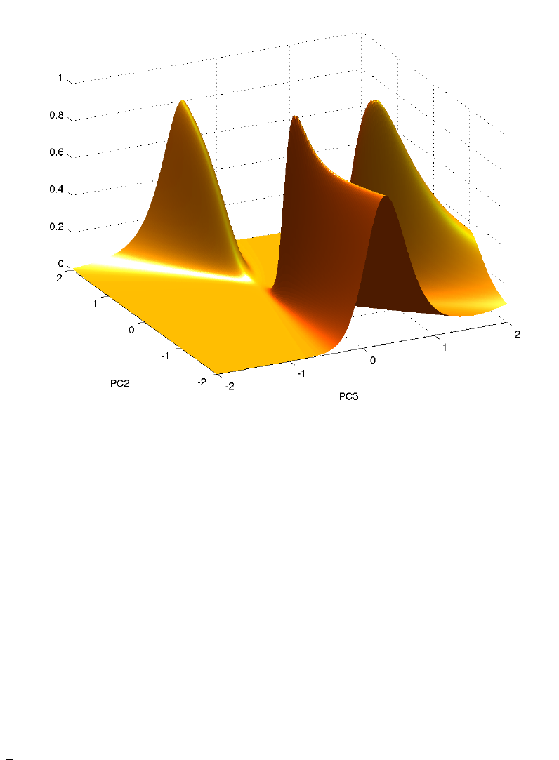
Figure 2: Likelihood Ratio Tests of the Autonomy Restriction under
P
. This figure reports
the p-values of the likelihood ratio test of whether a particular linear combination of yields,
β · P
t
, is autonomous under
P
, plotted against the loadings of PC2 and PC3. The loading of
PC1 is one minus the loadings on PC2 and PC3 (
β
(1) = 1
− β
(2)
− β
(3)). PC1, PC2, and
PC3 are scaled to have in-sample variances of one.
each potential volatility instrument
β · P
t
, we re-estimate the regression in (26) under the
constraint that
β
is a left eigenvector of
K
Q
1,∆
. As is seen in the previous exercise, the resulting
likelihood ratios reveal whether or not the volatility instrument considered is consistent with
the admissibility constraint A(Q).
Although we do not strictly observe the risk neutral forecasts
E
Q
t
[
P
t+∆
] for stochastic
volatility models due to the presence of convexity effects, we use a model-free approach to
obtain very good approximation. The insight again is that risk-neutral expectations are, up
to convexity, observed as forward rates. The
n
-year forward rate that begins in one month,
f
∆,n
t
=
1
n
((n + ∆)y
n+∆,t
− ∆r
t
) is, up to convexity effects:
f
∆,n
t
≈ E
Q
t
[y
n,t+∆
] (27)
where
y
n,t
denotes
n
-year zero yield observed at time
t
. Thus we can use (27) to approximate
E
Q
t
[
y
n,t+∆
] whereby we simply ignore any convexity terms. This approximation is reasonable
17
for two reasons. First, Jensen terms are typically small. Second, notice that since our primary
interest is not in the level of expected-risk neutral changes but in their variation (as captured
by
K
Q
1,∆
), it is only changes in stochastic convexity effects that will violate this approximation.
Thus to the extent that changes in convexity effects are small this approximation will be
valid for inference of K
Q
1,∆
.
Using this method, we extract observations on
E
Q
t
[
y
n,t+∆
] from forward rates which we
can then convert into estimates of
E
Q
t
[
P
t+∆
] using the weighting matrix
W
. We denote this
approximation of E
Q
t
[P
t+∆
] by P
f
t
. Whence regression (26) translates into:
P
f
t
= constant + K
Q
1,∆
P
t
+ noise. (28)
Regression (28) draws a nice analogy to the time series VAR(1) of (25) that we use in
examining
A
(
P
). Importantly, as this regression can be implemented completely independently,
abstracting from any time series considerations, it serves as a stand-alone assessment of
A
(
Q
),
up to the validity of our convexity approximation approach. Notably, (28) makes clear the
(essentially) contemporaneous nature of the estimation of
K
Q
1,∆
. Since
P
t
explains virtually all
contemporaneous yields and forwards (and thus portfolios of forwards such as
P
f
t
), the
R
2
’s
of (28) are likely much higher than those for the time series VAR(1) at the monthly frequency.
Therefore we expect much stronger identification for
K
Q
1,∆
. Intuitively, although we observe
only a single time series under the historical measure with which to draw inferences, we
observe repeated term structures of risk-neutral expectations every month and this allows us
to draw much more precise inferences.
Figure 3 plots the p-values for this test of the restrictions of various instruments to be
autonomous under
Q
. In stark contrast to Figure 2 and in accordance with our intuition,
we see that the risk-neutral measure provides very strong evidence for which instruments
are able to be valid volatility instruments. Most potential volatility instruments are strongly
ruled out with p-values essentially at zero. Thus, our results here suggest that were it only
up to
A
(
P
) and
A
(
Q
) to decide which volatility instrument to use, the latter would almost
surely be the dominant force, with the remaining degrees of freedom being the sign choice and
choosing which of the
N
left eigenvectors of
K
Q
1,∆
is the volatility instrument. This evidence
suggests that the no arbitrage restrictions can potentially have very strong impact in shaping
volatility choices.
Left open by the model-free nature of our analysis in this section is, among other things,
the possibility that the defining property of the volatility factor (
β
should match
M
2
) can be
powerful enough that it might dominate
A
(
Q
) at identifying potential volatility instruments.
We take up an in depth examination of this possibility in the next section.
5 Comparison of Gaussian and Stochastic Volatility
Models
To understand the contribution of matching
M
2
on the identification of the volatility loadings
β
, we estimate and compare the (Gaussian)
A
0
(
N
) models with stochastic volatility models.
18

Figure 3: Likelihood Ratio Tests of the Autonomy Restriction under
Q
. This figure reports
the p-values of the likelihood ratio test of whether a particular linear combination of yields,
β · P
t
, is autonomous under
Q
, plotted against the loadings of PC2 and PC3. The loading of
PC1 is one minus the loadings on PC2 and PC3 (
β
(1) = 1
− β
(2)
− β
(3)). PC1, PC2, and
PC3 are scaled to have in-sample variances of one.
19

N = 4 N = 3
A
0
(N)
0.998 0.027 0.032 0.014 0.997 0.028 0.025
-0.007 0.957 -0.128 -0.042 -0.003 0.954 -0.098
-0.010 0.006 0.895 -0.080 -0.005 -0.002 0.928
-0.009 -0.009 -0.085 1.007
A
1
(N)
0.999 0.027 0.030 0.013 0.998 0.028 0.024
-0.005 0.959 -0.123 -0.037 -0.002 0.955 -0.097
-0.010 0.006 0.902 -0.075 -0.005 -0.000 0.931
-0.006 -0.007 -0.079 1.018
A
2
(N)
0.998 0.028 0.031 0.013 0.997 0.029 0.025
-0.005 0.956 -0.125 -0.040 -0.002 0.954 -0.099
-0.009 0.003 0.899 -0.077
-0.005 -0.002 0.929
-0.005 -0.012 -0.080 1.010
Regression
0.998 0.027 0.029 0.014 0.997 0.027 0.025
-0.008 0.957 -0.118 -0.041 -0.003 0.958 -0.098
-0.011 0.005 0.905 -0.077 -0.006 0.007 0.925
-0.016 -0.006 -0.065 0.987
Table 1: K
Q
1,∆
Estimates.
Clearly, matching
M
2
is relevant only in the latter and not the former. Since the
A
0
(
N
)
models are affine models, the one month ahead conditional expectation of yields portfolios
P
also take an affine form. Thus for both Gaussian and stochastic volatility models, we can
write:
E
Q
t
[
P
t+∆
] =
constant
+
K
Q
1,∆
P
t
under the risk neutral measure. Of particular interest
is the estimates of the monthly risk-neutral feedback matrix,
K
Q
1,∆
, implied by these models.
As we will show in this section, estimates of
K
Q
1,∆
are highly similar across these models.
This suggests that the role of stochastic volatility (matching
M
2
) is inconsequential for the
estimation of
K
Q
1,∆
. Thus identifying volatility instrument (
β
) is simply limited to making
the choice of which left eigenvector of
K
Q
1,∆
and its sign can best match
M
2
. We use the same
dataset as in the preceding section and note that all of our results remain fully robust for a
shortened sample period that excludes the Fed experiment regime.
5.1 Comparison of K
Q
1,∆
estimates
We estimate
A
M
(
N
) models, with
M
= 0
,
1
,
2 and
N
= 3
,
4, and then rotate the state
variables into low order yield PCs. For estimation, we assume these PCs are priced perfectly
while higher order PCs are observed with i.i.d. errors. JLS show that this assumption is
innocuous as it is likely to deliver estimates close to those obtained by Kalman filtering where
all yields portfolios are observed with errors. Estimation details and full parameter estimates
are deferred to Appendix C.
20

Table 1 reports the estimates of
K
Q
1,∆
implied by these models. Recall the defining property
of
K
Q
1,∆
given by equation (26) in which
K
Q
1,∆
is informative about how
P
t
forecasts
P
t+∆
under the risk neutral measure. Since for each
N
,
P
t
is characterized by the same loading
matrix
W
(that corresponds to the first
N
PCs of bond yields) across all models, it follows
that
K
Q
1,∆
estimates are directly comparable across all models with the same number of
factors
N
. Focusing first on the two models
A
0
(3) and
A
1
(3), the two estimates of
K
Q
1,∆
are
strikingly close: most entries are essentially identical up to the third decimal place. This
evidence indicates that the identification by the cross-sectional information (and possibly
other moments shared between the
A
0
(3) and
A
1
(3) models) for the parameter
K
Q
1,∆
seems
overwhelmingly stronger than the restrictions coming from matching
M
2
. Enriching the
volatility structure to
M
= 2 does not overturn this observation: the
K
Q
1,∆
estimate implied by
the A
2
(3) model remains essentially identical. Additionally, changing the number of factors
to
N
= 4 (results also reported Table 1) or
N
= 2 (results not reported) does not alter our
observation.
We have argued that variation in the one month ahead risk-neutral expectations, as
determined by
K
Q
1,∆
, is well approximated by the regression based estimate of (28). This
estimate can be further improved by simple steps that take into account the affine structure
of bond yields. Specifically up to convexity effects, the affine structure of bond yields implies
that:
˜
B
n+∆
= K
Q
1,∆
˜
B
n
+
˜
B
∆
where
˜
B
n
denotes the unannualized loadings of
n
-year zero yields on
P
t
. This suggests we
can recover
K
Q
1,∆
in two steps. First, we project yields of all maturities onto the states
P
t
to
recover the loadings
˜
B
n
.
17
Second, an estimate of
K
Q
1,∆
is obtained by projecting
˜
B
n+∆
−
˜
B
∆
onto
˜
B
n
(allowing for no intercepts).
18
As can be viewed from the last panel of Table 1, this
model free estimate of
K
Q
1,∆
come strikingly close to estimates obtained from the no arbitrage
models. This evidence suggests that the cross-sectional information
alone
is sufficient to pin
down the risk-neutral feedback matrix, and this identification is so strong that information
from other constraints imposed by the models seems irrelevant.
Given the estimates of
A
M
(
N
) models, we are able to confirm that the convexity effects
on yield loadings are negligible. Specifically, holding
N
fixed, varying
M
, and thereby varying
the degree of convexity effects due to the presence of stochastic volatility, is completely
inconsequential for the yield loadings implied by different models. Graphs (not reported) of
yield loadings on
P
t
plotted against the corresponding maturities (up to ten years) implied
by A
0
(N), A
1
(N), and A
2
(N) are virtually indistinguishable.
The observed invariance property of
K
Q
1,∆
estimates has a number of implications. First,
as stated previously, this allows us to pin down the potential volatility instruments using the
cross-section of yields due to the admissibility constraint. Essentially the volatility instrument
is free in terms of the sign but must be one of the left eigenvectors of
K
Q
1,∆
which can be
17
To obtain yields for the full range of maturities from the small set of maturities used in estimation, we
can use simple interpolation techniques such as the constant forward bootstrap or simply a cubic spline.
18
de los Rios (2013) develops a similar regression-based approach to obtain estimates of K
Q
1,∆
.
21

computed accurately from either the cross-sectional regression or from estimation of the
A
0
(
N
) model which has constant volatility and can be estimated quite quickly as shown in
JSZ.
This observation also shows that, in some regards, the estimation of the no arbitrage
A
1
(
N
) model is more tractable than estimate of the F
1
(
N
) model. In the case of the Gaussian
models the opposite holds: the factor model is trivial to estimate as it amounts to a set of
ordinary least squares regressions while the no arbitrage model is slightly more difficult to
estimate due to the non-linear constraints in the factor loadings. In the stochastic volatility
models, the admissibility conditions require a number of non-linear constraints in order
to ensure that volatility remains positive. The no arbitrage model essentially determines
the volatility instrument up to sign and choice of eigenvector. This actually simplifies the
estimation since it reduces the set of non-linear constraints that need to be imposed.
The observation that
K
Q
1,∆
estimates are nearly invariant across Gaussian and stochastic
volatility models leads us to the surprising conclusion that the
A
0
(
N
) model with
constant
volatility
allows us to essentially identify (up to choice of which eigenvector) the source of
stochastic volatility in the
A
1
(
N
) model. We provide an illustration of this point in the next
subsection.
5.2 Volatility information revealed by the Gaussian model
Despite the similarity, the estimates of
K
Q
1,∆
reported in Table 1 still exhibit slight numerical
differences. It is possible these small numerical differences might become more significant
in terms of the left eigenvectors and thus among model implied volatility instruments. To
show that this is not the case, we carry out the following exercise. Starting with the
K
Q
1,∆
estimate by the
A
0
(3) model, we form three potential volatility instruments from the three
left eigenvectors of
K
Q
1,∆
and then pick out the instrument with most predictive content
for volatility. Specifically, we first project the level factor,
P
1,t+∆
, onto
P
t
to obtain the
forecast residuals and then choose the volatility candidate with most predictive content for
the squared residuals. This way, from the
A
0
(3) model, we can have a “guess” for what the
volatility instrument of the
A
1
(3) model looks like even before we actually estimate the
A
1
(3)
model. Finally, we compare this “guess” to the actual volatility instrument implied by the
A
1
(3) model.
Table 2 reports the adjusted
R
2
statistics (in percentage) of regressions in which each
potential volatility instrument is used to predict the squared residuals of the level factor.
Evidently, one of the instruments clearly dominates the others at all forecasting horizons
from one to twelve months. Comparing this dominant instrument to the actual volatility
factor of the
A
1
(3) model results in a striking correlation of one. To see this more visually, we
plot these two volatility instruments, normalized to have the same scaling and intercepts,
19
in Figure 4. Clearly, the
A
0
(3)’s “guess” is very accurate as the two graphs are right on top
of one another.
19
Specifically, in constructing both volatility instruments, we drop the intercepts and scale the loading on
the level factor (β(1)) to one.
22

Horizon Instrument 1 Instrument 2 Instrument 3
1 9.35 -0.00 0.58
2 8.84 -0.21 -0.16
3 8.66 0.92 2.17
4 7.32 0.96 2.55
5 6.51 0.50 1.84
6 6.04 -0.24 0.12
7 5.28 -0.07 0.57
8 4.71 -0.24 0.01
9 4.87 0.33 1.26
10 4.59 0.51 1.66
11 4.27 0.51 1.77
12 4.21 0.03 0.95
Table 2:
R
2
(in percentage) predicting squared residuals in forecasting the level factor by
the three potential volatility instruments implied by the
A
0
(3) model. Instruments 1, 2, 3
are formed from the left eigenvectors of the
K
Q
1,∆
matrix, corresponding to the eigenvalues
ordered from highest to lowest.
1970 1975 1980 1985 1990 1995 2000 2005 2010
0.04
0.06
0.08
0.1
0.12
0.14
0.16
0.18
A
0
(3) guess
A
1
(3)
Figure 4: Volatility instrument “guessed” by the
A
0
(3) model and the actual volatility factor
implied by the
A
1
(3) model. The volatility instrument is normalized as
β · P
t
where
β
(1) is
scaled to one.
23
This exercise and the content of the previous subsection clearly reveal the respective roles
of the cross-sectional and time series information in shaping the choice of volatility instrument
in an
A
1
(3) model. The cross-sectional information pins down the risk-neutral feedback
matrix
K
Q
1,∆
. The identification seems so strong that time series constraints from matching
M
1
(
P
) and
M
2
appear inconsequential. Regardless of whether the time series constraints are
applied (in the
A
1
(3) model) or not (in the
A
0
(3) model), the estimates of
K
Q
1,∆
seem largely
unaffected. The precise estimate of
K
Q
1,∆
together with
A
(
Q
) dramatically reduces the choice
of potential volatility instruments from an uncountably infinite set to a discrete choice among
the
N
left eigenvectors of
K
Q
1,∆
. This is the very sense in which a constant volatility model
such as the
A
0
(
N
) model can reveal volatility information of stochastic volatility models.
The
A
0
(
N
) model pins the optimal volatility instrument to be one of the
N
left eigenvectors,
but it does not determine exactly which one. It is the role of the time series constraints in
picking the left eigenvector (and its sign) that best matches M
1
(P) and M
2
.
6 No Arbitrage Restrictions
In this section, we show that the clear distinction of the roles of cross-section and time
series information in determining the volatility of no arbitrage models can have important
implications for dynamic term structure models. Specifically, we reconsider the puzzling result
of Dai and Singleton (2002). They show that while Gaussian models are able to replicate the
deviations from the expectation hypothesis found in the data, affine term structure models
with stochastic volatility are unable to match the patterns found in the data. This failure
may potentially be due to the tension between first and second moments. However, we show
that the stochastic volatility factor model (where the first and second moment tension still
applies) is able to match deviations from the expectations hypothesis. This demonstrates
that the tension created by also matching
M
1
(
Q
) in addition to
M
1
(
P
)and
M
2
is what drives
the failures of the stochastic volatility models demonstrated by Dai and Singleton (2002).
These results, together with our previous results, show that recent results about the
irrelevancy of no arbitrage restrictions in Gaussian models do not extend to affine models
with stochastic volatility. For example, Duffee (2011), Joslin, Singleton, and Zhu (2011), and
Joslin, Le, and Singleton (2012) all show that no arbitrage is nearly irrelevant in Gaussian
dynamic term structure models on a number of dimensions. In contract, for the case of
stochastic volatility models, the no arbitrage constraints on the factor model has material
effects for both first and second moments.
6.1 Expectation hypothesis
A generic property of arbitrage-free dynamic term structure models is that risk-premium
adjusted expected changes in bond yields are proportional to the slope of the yield curve.
Under the expectation hypothesis (EH), risk premiums are constant. This implies that the
24

coefficients φ
n
in the projections
P roj [y
n−∆,t+∆
− y
n,t
|y
n,t
− y
∆,t
] = α
n
+ φ
n
y
n,t
− y
∆,t
n − ∆
, for all n > ∆, (29)
should be uniformly ones under the EH. Campbell and Shiller (1991) shows robust evidence
that
φ
n
’s are significantly different from one and become increasingly negative for large
n
’s.
This puzzling pattern of
φ
n
’s, which can be observed in Figure 1 for our sample period, has
become one of the most studied empirical phenomena for the last twenty years.
Dai and Singleton (2002) show that constant volatility models are not “puzzled” by this
pattern and that the population coefficients
φ
n
implied by estimated
A
0
(
N
) models very
closely match their data counterparts. However, Dai and Singleton (2002) show a stark
contrast for the canonical models
A
M
(
N
) models with
M >
0 with stochastic volatility. Here
they find
φ
n
’s typically stay close to the unit line, thereby counter-factually implying that
the EH nearly holds.
What is behind the difference in performances of the Gaussian and stochastic volatility
models? To begin, it is worth noting that the loadings
φ
n
’s for all affine models (with or
without no arbitrage restrictions) can be written as:
φ
n
= (n − ∆)
(B
n−∆
K
1,∆
− B
n
)Σ(B
n
− B
∆
)
0
)
(B
n
− B
∆
)Σ(B
n
− B
∆
)
0
. (30)
where Σ denotes the unconditional covariance matrix of the time series innovations and
B
n
the loadings of the
n
-period yield
y
n,t
on the principal components of yields
P
t
. As
noted earlier, the loadings
B
’s are essentially identical across models with and without
stochastic volatility.
20
Furthermore, the covariance matrix Σ appears in both the numerator
and denominator of (30), thus its impact on
φ
n
is greatly dampened due to cancellation. This
essentially leaves the one-month ahead physical feedback matrix
K
1,∆
as the natural focus in
explaining the differences in φ
n
’s across the constant and stochastic volatility models.
One of the main findings of JSZ in the context of the Gaussian models is that no arbitrage
restrictions are irrelevant for models’ forecasting performance. Equivalently, estimates of the
one-month ahead physical feedback matrix
K
1,∆
from
A
0
(
N
) models are exactly identical to
those obtained from OLS regressions of
P
t+∆
on
P
t
and, thus, completely unaffected by no
arbitrage restrictions. Turning to the
A
1
(
N
) models, the concurrent presence of
A
(
P
) and
A
(
Q
) builds a strong link between the one-month ahead physical and risk neutral feedback
matrices:
K
1,∆
and
K
Q
1,∆
must share one common left eigenvector. To the extent that
K
Q
1,∆
is
very strongly pinned down by the cross-section information, it is likely to force the physical
feedback matrix
K
1,∆
to accept one of the
N
left eigenvectors of
K
Q
1,∆
as one of its own.
Due to this coupling of
K
1,∆
and
K
Q
1,∆
, the estimate of
K
1,∆
from the
A
1
(
N
) model is likely
strongly influenced by the no arbitrage restrictions and thus can be quite different from its
OLS counter-part.
20
In fact, these loadings are very close to those obtained from OLS regressions of yields of individual
maturities onto the pricing factors P
t
.
25

N = 4 N = 3
A
0
(N)
0.990 -0.009 -0.047 -0.017 0.990 -0.009 -0.047
0.010 0.955 -0.080 -0.032 0.010 0.955 -0.080
-0.002 0.010 0.799 0.030 -0.002 0.010 0.799
0.000 0.012 -0.012 0.627
A
1
(N)
0.990 0.015 0.002 -0.034 0.993 0.011 -0.035
0.004 0.975 -0.080 -0.099 0.006 0.973 -0.100
0.000 0.002 0.835 0.013 -0.001 -0.009 0.823
-0.006 0.001 -0.031 0.703
A
2
(N)
0.987 0.017 0.035 -0.004 0.992 0.015 0.009
-0.002 0.958 -0.083 -0.106 0.004 0.974 -0.075
0.002 0.013 0.870 0.052
0.013 0.011 0.902
0.001 0.020 -0.025 0.729
F
1
(N)
0.991 -0.013 -0.093 -0.010 0.997 -0.018 -0.081
0.006 0.962 -0.054 -0.045 0.002 0.965 -0.052
0.009 -0.012 0.867 0.048 0.005 -0.008 0.830
-0.009 0.022 0.003 0.715
F
2
(N)
0.994 -0.013 -0.086 0.028 0.998 -0.018 -0.056
0.005 0.962 -0.067 -0.070 0.005 0.965 -0.010
0.005 -0.012 0.876 0.032 0.004 -0.007 0.828
-0.003 -0.011 -0.027 0.702
Table 3: K
1,∆
Estimates
Table 3 reports estimates of
K
1,∆
for the
A
M
(
N
) models with
M
= 0
,
1
,
2 and
N
= 3
,
4.
The sample period is 1973 through 2007 and we note, again, that all of our results for a
shortened sample period that excludes the Fed experiment regime remain qualitatively similar.
Comparing the
A
0
(
N
) and
A
1
(
N
) models reveals one interesting difference: for both
N
= 3
and
N
= 4, the (1,2) entry of the feedback matrix, which governs how slope this period
forecasts level next month, is negative for the
A
0
(
N
) model but positive for the
A
1
(
N
) model.
A negative value for this entry means that higher slope leads to lower level and thus higher
return in the future whereas the opposite is true for a positive entry. As is well-known, the
Campbell and Shiller (1991) regression in (29) is equivalent to one in which future bonds’
excess returns are projected onto a measure of slope:
P roj[xr
n−∆
t+∆
|y
n,t
− y
∆,t
] = (1 − φ
n
)(y
n,t
− y
∆,t
) (31)
where
xr
n−∆
t+∆
denotes one-month excess returns on the
n −
∆ period bond, realized at time
t
+ ∆. Combining with the established empirical fact that the Campbell and Shiller (1991)
loadings
φ
n
’s are always below one (and mostly negative), (31) clearly reveals that higher
slope must be followed by higher returns. It follows that the positive (1,2) entry of the
26
feedback matrix, which counter-factually implies that higher slope must be followed by lower
returns, is likely the key weak point of the
A
1
(
N
) models. Moreover, the same weakness also
applies to the
A
2
(
N
) models as the (1,2) entries for these models are also similarly positive.
To examine whether the no-arbitrage restrictions are indeed forcing the physical feedback
matrix of the stochastic volatility models to admit these counter-factual values, we estimate
the
F
M
(
N
) models established in Section 3. Recall that these are the counter-parts to the
A
M
(
N
) models with the no-arbitrage restrictions, and thus the “first moments” restrictions
through
A
(
P
), completely relaxed. We use the same sample period (1973 through 2007)
and the same set of yields in estimation, thus the estimated
F
M
(
N
) and
A
M
(
N
) models are
directly comparable. Examining the reported values of the
K
1
matrix reported in the last
two panels of Table 3, for all four
F
M
(
N
) models (M=1,2 and N=3,4) the (1,2) entry of the
feedback matrix is negative.
Although a negative (1,2) entry should now allow slope to forecast level with the right
sign, the key question is whether the
F
M
(
N
) models, without no arbitrage restrictions, can
produce loadings
φ
n
’s that match up with the Campbell and Shiller (1991) regression (31)
in the data. The answer to this question is a definite yes! Examining the pattern of the
loadings
φ
n
implied by the
A
1
(3) and
A
2
(3) models in Figure 1, we find the well-known result
of Dai and Singleton (2002) in which these stochastic volatility models have a long way to go
in matching the empirical Campbell and Shiller (1991) regression coefficients. Nevertheless,
once the no arbitrage restrictions are dropped and the the
A
1
(3) and
A
2
(3) models turn into
the corresponding
F
1
(3) and
F
2
(3) models, the model-implied
φ
n
’s now become extremely
close to their empirical counter-parts, arguably as close as those loadings implied by the
A
0
(3) model. A graph (not reported) for four factor models shows very similar results.
In short, Figure 1 constitutes convincing evidence that the no arbitrage restrictions, and
in particular needed to match
M
1
(
Q
), seem directly behind the failure of the
A
M
(
N
) models
for
M >
0 in explaining the deviations from the EH. In stark contrast, the admissibility
restriction
A
(
P
) under the physical measure – present in both the
A
M
(
N
) as well as
F
M
(
N
)
models – appears largely inconsequential for a model’s ability in matching the deviations
from the EH.
6.2 Why does imposing no-arbitrage lead to slope predicting level
with a positive sign?
Whereas it seems clear the presence of no-arbitrage forces slope to predict level with a
positive sign, thereby impairing no arbitrage stochastic volatility models’ ability to match
the empirical Campbell and Shiller (1991) regression coefficients, the exact mechanism is not
obvious. To shed light on this, and with an emphasis on intuition, we focus on the
A
1
(
N
)
models and present two heuristic results. First, we show that as long as the risk-neutral
dynamics of the non-volatility factors are not too close to being explosive, the loadings of the
volatility factor on the level and slope factors (
β
(1) and
β
(2)) will have the same sign. Second,
we show that, given the tendency of the volatility factor to be relatively more persistent than
the slope factor, the sign constraint on
β
(1) and
β
(2) necessarily causes slope to predict level
27

with a positive sign.
To see the former result in the most simplified manner, let’s focus on the two-factor model
A
1
(2) and think of the level and slope factors simply as the one-year yield, and the spread
between the ten-year and one-year yield, respectively. We can show in Appendix A that the
volatility loadings (with the first entry normalized to one) can be written as:
β = (1, W
1
B
Q
X
(W
2
B
Q
X
)
−1
),
where
W
1
= (1
,
0),
W
2
= (
−
1
,
1). Furthermore, standard bond pricing calculations reveal that
B
Q
X
= ∆
1−e
λ
Q
X
(1−e
λ
Q
X
∆
)
,
1−e
10λ
Q
X
10(1−e
λ
Q
X
∆
)
0
where
λ
Q
X
denotes the risk-neutral eigenvalue corresponding
to the non-volatility factor as in (14). A few algebraic steps show that :
β(2) = W
1
B
Q
X
(W
2
B
Q
X
)
−1
=
1 − e
λ
Q
X
1 − e
λ
Q
X
−
1−e
10λ
Q
X
10
. (32)
Clearly, as long as
λ
Q
X
≤
0, or equivalently the non-volatility factor is stationary, both the
numerator and the denominator of the right hand side of (32) are positive. Therefore we can
make the following statement for the A
1
(2) model:
1.
As long as the non-volatility factor is
Q
-stationary, the loading of the volatility factor
on slope will always be of the same sign as the loading on level.
2.
To the extent that the loading of volatility on level is generally positive, it implies that
the loading on slope is also positive.
Similar results hold up for more general loadings of the level and slope factors and for
the
A
1
(3) model. Adopting the loadings
W
that correspond to the lower order yield PCs,
we roam over the possible values of
λ
Q
X
≤
0 for both cases
N
= 2 and
N
= 3 and plot in
Figure 5 the corresponding values of 1 +
log
(
β
(2)) (again with
β
(1) normalized to one). Note
that this transformation, chosen for better scaling of the graphs, is positive if and only if
β
(2) is positive. As can be seen clearly from the graphs,
β
(2) is always positive, implying
that both level and slope will load with the same sign in the volatility instrument of both the
A
1
(2) and A
1
(3) models.
Turning to the second result, let’s start by noting that the normalized volatility factor of
the A
1
(2) model can be written as:
V
t
= β · P
t
= L
t
+ β(2)S
t
(33)
where
L
is the level,
S
is the slope, and
β
(2) is positive. Now the admissibility restriction
under the physical measure requires that only V
t
can forecast V
t+∆
, or equivalently:
E
t
[V
t+∆
] = constant + ρ
V
V
t
. (34)
28

0.5 0.55 0.6 0.65 0.7 0.75 0.8 0.85 0.9 0.95 1
0
0.5
1
1.5
2
2.5
3
A
1
(2)
exp(h
Q
X
6)
log(1+`(2))
(a) A
1
(2)
0.5 0.55 0.6 0.65 0.7 0.75 0.8 0.85 0.9 0.95 1
0
0.5
1
1.5
2
2.5
exp(h
X,2
Q
6)
log(1+`(2))
A
1
(3)
exp(h
X,1
Q
6)=0.75
exp(h
X,1
Q
6)=0.85
exp(h
X,1
Q
6)=0.95
(b) A
1
(3)
Figure 5: log(1 + β(2)) for various values of λ
Q
X
.
Substitute (33) into (34) and evaluate the one month forecast of the level factor, we
obtain:
E
t
[L
t+∆
] = constant + ρ
V
L
t
+ β(2)(ρ
V
S
t
− E
t
[S
t+∆
]). (35)
Assuming slope forecasts future slope with a coefficient of
ρ
S
,
21
then it follows from (35) that
slope forecasts future level with a coefficient of
β(2)(ρ
V
− ρ
S
).
Due to the sign restriction
β
(2)
>
0, established above, the sign with which slope forecasts
level is dependent on the difference between
ρ
V
, the persistence of the volatility factor, and
ρ
S
. Empirically, due to well known volatility level effect, the volatility factor is typically
quite persistent. In contrast, the slope factor operates at a relatively higher frequency. This
suggests that
ρ
S
, which is closely related to the persistence of the slope factor, is likely much
smaller than ρ
V
, thus requiring slope to forecast level with a positive coefficient.
7 Risk price specification and identification of the volatil-
ity factor(s)
Within the class of
Q
-affine term structure models, many different specifications for the market
prices of risks have been proposed. Starting with the completely affine setup formalized by
Dai and Singleton (2000), we have seen more flexible affine forms such as Duffee (2002),
Cheridito, Filipovic, and Kimmel (2007), as well as non-affine forms such as Duarte (2004).
Depending on the risk-price specifications, the physical dynamics can be affine or non-affine.
21
To be more precise, E
t
[S
t+1
] = constant + ρ
S
S
t
+ ρ
SL
L
t
but we focus only on the S
t
term.
29

A
0
(3) Duarte
1
(3) Diag
1
(3)
0.997 0.028 0.025 0.998 0.028 0.024 0.998 0.028 0.024
-0.003 0.954 -0.098 -0.002 0.955 -0.097 -0.002 0.955 -0.098
-0.005 -0.002 0.928 -0.005 -0.000 0.931 -0.005 -0.000 0.930
Table 4: K
Q
1,∆
Estimates
Nonetheless, a common thread through all of these different modelling choices is the fact
that the risk-neutral dynamics of the underlying states remain affine and, importantly, free
of artificial constraints beyond those that guarantee admissibility.
Recall from Section 5 that our regression-based estimates of the risk-neutral feedback
matrix
K
Q
1,∆
, which are completely independent of any physical dynamics, are quite close
to estimates implied by the
A
M
(
N
) models. It is therefore very likely that the risk neutral
feedback matrix
K
Q
1,∆
will be very strongly identified regardless of their risk price specifica-
tions. Moreover, specializing to models with one volatility factor, due to
A
(
Q
), the strong
identification of
K
Q
1,∆
translates into a virtually discrete choice of the volatility instruments
from the
N
left eigenvectors of
K
Q
1,∆
. As is seen earlier, given the
N
left eigenvectors, the
choice of which volatility instrument seems to rest on the matching of
M
2
and much less on
the functional form of risk prices. We therefore conjecture that the volatility factor implied
by these models is likely highly similar across different risk price specifications.
To confirm our conjecture, we use the same data used earlier to estimate two term
structure models with one volatility factor for
N
= 3 with different risk price specifications.
The first adopts the non-affine approach of Duarte (2004) to include a square-root term in
the risk price of the volatility factor. The second restricts the conditional feedback matrix
corresponding to the PC yields portfolios to be diagonal under the physical measures. Similar
diagonal restrictions have been considered by Joslin, Le, and Singleton (2012), among others.
We refer to these models as Duarte
1
(3) and Diag
1
(3), respectively.
As is evident from Table 4, the risk neutral feedback matrices implied by
Duarte
1
(3)
and
Diag
1
(3) are virtually identical and are extremely close to the
K
Q
1,∆
matrix implied by
the constant volatility model
A
0
(3) (which is shown earlier to be very close to that implied
by the
A
1
(3) model). Comparing the volatility factors implied by
Duarte
1
(3) and
Diag
1
(3)
in Figure 6 clearly reveals that these volatility factors are virtually indistinguishable. Very
similar results (not reported) are obtained for four factor models and for a shortened sample
period that excludes the Fed regime. In short, we find strong evidence that altering the price
of risk specification is relatively inconsequential for the identification of volatility.
8 Extensions
In this section, we show how our results extend to the case of multiple volatility factors and
unspanned stochastic volatility. As before, this tension arises because of the relationship
30

1970 1975 1980 1985 1990 1995 2000 2005 2010
0.04
0.06
0.08
0.1
0.12
0.14
0.16
0.18
A
1
(3)
Duarte
1
(3)
Diag
1
(3)
Figure 6: Volatility factor (
β·P
t
where
β
(1) is scaled to one) implied by the
A
1
(3),
Duarte
1
(3),
and Diag
1
(3) models.
between the left eigenspaces of the feedback matrices under
P
and
Q
. Additionally, new
conditions arise because of requirements of positive feedback amongst CIR factors. We also
show how our results extend to the case of unspanned stochastic volatility.
8.1 Multiple volatility factors
In an
A
M
(
N
) model, as
M
rises relative to
N
, the restriction that the univariate volatility
factor is an autonomous process weakens to the requirement that the
M
-dimensional volatility
process is autonomous. This allows for richer feedback among the factors. While the conditions
are weaker in this sense, new conditions arise where now feedback amongst the volatility
factors must be positive. Additionally, such factors are now required to be independent.
Although the proof of the results that we state below are generally direct, we omit them due
to their tedious nature.
An A
M
(N) model has a latent factor representation as
dZ
t
= (K
0
+ K
1
Z
t
) dt + +
p
Σ
0
+ Σ
1,1
Z
t1
+ . . . + Σ
1M
Z
t,M
dB
t
(36)
31

with r
t
= ρ
0
+ ρ
1
· X
t
and the admissibility requirements:
K
0i
≥
1
2
Σ
1,i,ii
, i ≤ M, (37)
K
1,ij
≥ 0, i, j ≤ M, i 6= j, (38)
K
1,ij
= 0, i ≤ M < j, (39)
Σ
0,ii
= 0, i ≤ M, (40)
Σ
1,i,jj
= 0, i, j ≤ M, i 6= j, (41)
and Σ
0
,
Σ
1
, . . . ,
Σ
M
are positive semi-definite symmetric matrices. Similar relations apply for
the risk-neutral dynamics. As before we have the relation
y
t
= A
Q
Z
+ B
Q
Z
Z
t
, (42)
where A
Q
Z
and B
Q
Z
are dependent on the underlying parameters.
When
M >
1 there will be multiple volatility instruments given by a set of vectors
B
=
{β
1
, β
2
, . . . , β
M
}
. As before, we will require that under both the historical and risk-
neutral measures there are CIR-type factors which do not have any feedback from the
conditionally Gaussian factors. In the
A
1
(
N
) case, this required that
β
1
is a left eigenvector
of
K
1
and
K
Q
1
. For the general case of
M ≥
1, we require that there exists
M
left eigenvectors
of
K
1
,
{e
1
, . . . , e
M
}
, and
M
left eigenvectors of
K
Q
1
,
{f
1
, . . . , f
M
}
so that the span of
B
is
the same of the span of both
{e
0
1
, . . . , e
0
M
}
and
{f
0
1
, . . . , f
0
M
}
.
22
This will give a direct tension
between first moments.
The conditions for no-feedback between conditionally Gaussian and CIR factors required
by (39) imply eigenvector restrictions that give rise to a tension between
M
1
(
P
) and
M
1
(
Q
).
The restriction of positive feedback among the CIR factors given by (38) also implies a tension
between
M
1
(
P
) and
M
1
(
Q
). To illustrate these tensions, let us consider the case of an
A
2
(2)
model. In this case, since M = N, the eigenvector conditions do not bind.
Suppose that
K
Q
1
has real eigenvalues
{λ
1
, λ
2
}
. with corresponding eigenvectors
{u
1
, u
2
}
.
Then
UK
Q
1
U
−1
=
diag
(
λ
1
, λ
2
) where
U
= [
u
0
1
, u
0
2
]. Straightforward but tedious computations
imply that the positive feedback conditions in (38) requires that Γ =
UK
1
U
−1
must satisfy
one of:
1. Γ
12
Γ
21
≥ 0, or
2. Γ
21
< 0 < Γ
12
and Γ
22
− Γ
11
> 2
√
−Γ
12
Γ
21
, or
3. Γ
12
< 0 < Γ
21
and Γ
11
− Γ
22
> 2
√
−Γ
12
Γ
21
.
Note that by our previous logic,
K
Q
1
is likely to be strongly identified by the cross-section
of yields and largely invariant to the choice of
M
. Therefore
U
should be estimated very
precisely. If one considers
U
to be fixed (i.e. estimated without error), then the conditions
22
Alternatively, we can characterize the relation that the exists a single fixed matrix
U
so that for each
i
,
both (i) K
0
1
(Uβ
i
) is in the span of B and (ii) (K
Q
1
)
0
(Uβ
i
) is in the span of B.
32
above translate into quadratic constraints on
K
1
. This is the new tension between
M
1
(
P
)
and M
1
(Q) not present in A
1
(N) models.
In addition, the tensions with
M
2
become more pronounced. To see this, suppose that
{c
1
· P
t
, c
2
· P
t
}
have uncorrelated innovations. That is, the covariance matrix of innovations
to
CP
t
, where
C
= [
c
0
1
, c
0
2
]
0
, is diagonal. Then it must be that
CK
1
C
−1
and
CK
Q
1
C
−1
has
non-negative off-diagonal elements. Again taking the extreme example that
K
Q
1
is estimated
without any error, this will impose a restriction on which possible linear combinations of
P
t
are uncorrelated.
8.2 Unspanned stochastic volatility
With some modifications, our results also apply in models with unspanned stochastic volatility
as in Collin-Dufresne and Goldstein (2002) and Bikbov and Chernov (2009), among others.
We now discuss these results for the case of one or more stochastic volatility factors as well
as for the cases with purely unspanned stochastic volatility or a mixture of spanned and
unspanned stochastic volatility. Similar results would apply in cases with unspanned risk
such as inflation risk (see, e.g. Chernov and Mueller (2009)), provided additional data is
available to price this risk such as inflation swaps.
In the case of an
A
1
(
N
) model with unspanned stochastic volatility, the tension implies
that volatility is an autonomous process under
M
1
(
P
) and
M
1
(
Q
). The clean separation of
yields and volatility will imply that our results are informative only about volatility and will
require that volatility is an autonomous process, which is well understood in the literature.
For example, Almeida, Graveline, and Joslin (2011) find correlations between yield curve
factors and volatility measures as high as 84% while Jacobs and Karoui (2009) find
R
2
as
high as 75%.
When
M >
1, several possibilities arise. Joslin (2013a) develops an
A
2
(
N
) model
where there are both spanned and unspanned stochastic volatility. Such a model would be
consistent with the moderate
R
2
(but less that 100%) that are available from projecting
volatility/variance measures onto the yield curve. Our existing results will apply directly
to the spanned component of volatility. For example, the possible choices for the spanned
instrument for volatility will be determined by
K
Q
1
. Moreover, spanned and unspanned
volatility factors will follow an
A
2
(2) process. The previous discussion of
A
2
(2) models will
now apply. In this case,
M
1
(
P
) and
M
1
(
Q
) will be determined by actual and risk-neutral
forecasts of volatility. Risk-neutral forecasts of volatility will now be identified by a cross-
section of option prices instead of bond prices. For example, if
V
t
= (
V
span
t
, V
unspan
t
) and
CV
t
has uncorrelated innovations, then our results in Section 8.1 show that the risk-neutral and
actual forecasts will have to satisfy a number of constraints.
Another alternative is to have a model with multiple unspanned stochastic volatility
factors. Joslin (2013a) and Trolle and Schwartz (2009) show how to construct such models.
In this case, our results regarding
A
2
(2) models (and more generally
A
N
(
N
)) will apply
to the volatility factors. Thus, again, there will be tensions as we have outlined between
risk-neutral and actual forecasts of volatility as well as the volatility of volatility. Moreover,
our logic would generally apply to multiple unspanned volatility factors where the risk-neutral
33
dynamics could be identified by options as in Carr, Gabaix, and Wu (2009).
9 Conclusion
In the context of no arbitrage affine term structure model with stochastic volatility, we
document a strong tension between the first moments of bond yields under the time series and
risk neutral measures. We show that, beyond other types of tensions documented so far in
the existing literature, this tension is key in understanding important economic implications
of no-arbitrage affine models with stochastic volatility. In particular, this tension underlies
the well-known failure of the
A
M
(
N
) class of models in explaining the deviations from the
EH in bond data.
Our primary results are driven by the fact that an affine drift requires a number of
constraints in order to assure that volatility stays positive. A number of alternative models
could be considered. First, one could consider a model with unspanned or nearly unspanned
volatility. This, however, can only partially counteract our results in the sense that the
projection of volatility onto yields must still mathematically be a positive process. So several
of our insights maintain. Another possible model to consider is a model with non-linear drift.
That is, we can suppose that there is a latent state variable
Z
t
with the drift of
Z
t
linear
in
Z
t
without any constraints provided that volatility (or its instrument) is far from the
boundary. Near the zero boundary, the drift of the volatility may be non-linear in such a way
as to maintain positivity. Provided that the probability of entering this non-linear region is
small (under Q), similar pricing equation will be obtained as in the standard affine setting.
34
A Dependence of Volatility Loadings β and the Eigen-
values under Q
Our arguments in Section 3.3 rest on the approximation that convexity effects are negligible.
Although we confirm empirically that this approximation holds up in the data, we now
make our arguments more precise by showing that the volatility instrument
β
is in fact
completely determined by the (N − 1) eigenvalues given in λ
Q
X
. This can be seen as follows.
Let
P
(1)
t
=
W
1
y
t
(
P
(2)
t
=
W
2
y
t
) denote the first entry (entries two to N) of
P
t
where
W
1
(
W
2
)
refers to the first row (rows 2 to N) of
W
. Let
B
Q
V
and
B
Q
X
denote the yield loadings on
V
t
and
X
t
, respectively. Thus,
B
Q
V
corresponds to the first column, and
B
Q
Z
the remaining
columns of
B
Q
Z
. Notably, due to the block structure of the feedback matrix in (14) and the
fact that the non-volatility factor
X
t
does not give rise to Jensen effects, it can be shown
that B
Q
X
only depends on λ
Q
X
. Then we have,
P
(1)
t
= constant + W
1
B
Q
V
V
t
+ W
1
B
Q
X
X
t
P
(2)
t
= constant + W
2
B
Q
V
V
t
+ W
2
B
Q
X
X
t
.
This gives two equations and two unknowns, so we can subtract
W
1
B
Q
X
(
W
2
B
Q
X
)
−1
times the
second equation from the first equation to eliminate X
t
and obtain
P
(1)
t
− W
1
B
Q
X
(W
2
B
Q
X
)
−1
P
(2)
t
= constant + cV
t
,
where
c
is a constant. This shows directly that no arbitrage imposes the restriction (up to
scaling):
β = (1, −W
1
B
Q
X
(W
2
B
Q
X
)
−1
). (43)
We see that the volatility instrument is in fact determined entirely by
λ
Q
X
. Coupled with our
reasoning earlier that
λ
Q
X
should be strongly pinned down in the data, it is clear that the
volatility instruments are heavily affected by the no arbitrage restrictions. Equation (43) also
makes clear the nature of the (close) relationship between the volatility instrument and yield
loadings discussed earlier.
B A Canonical Form for Discrete-Time Term Struc-
ture with Stochastic Volatility
In this section, drawing on the construction in Le, Singleton, and Dai (2010) (LSD), we lay out
canonical forms for discrete-time affine term structure models with stochastic volatility. As is
shown by LSD, for monthly data, these provide very good approximation to the continuous
time A
M
(N) models in the main text.
We start by assuming that the economy is fully characterized by the
N
-variate state
vector
Z
t
= (
V
0
t
, X
0
t
)
0
where
V
t
is a strictly positive
M
-variate volatility process and
X
t
is
conditionally Gaussian. The time interval is ∆.
35

B.1 Risk-neutral dynamics and bond pricing
Under Q, our states follow:
V
t+∆
|V
t
∼ CAR(ρ
Q
, c
Q
, ν
Q
), (44)
X
t+∆
∼ N(K
Q
1V,∆
V
t
+ K
Q
1X,∆
X
t
, Σ
0,∆
+
M
X
i=1
Σ
i,∆
V
i,t
), independent of V
t+∆
(45)
r
t
= r
∞
+ ρ
0
V
V
t
+ ι
0
X
t
. (46)
CAR denotes a compound autoregressive gamma process. See LSD for more details.
Each CAR process is fully characterized by three non-negative parameters:
ρ
Q
(
M × M
),
c
Q
(M × 1), and ν
Q
(M × 1). The Laplace transform for a CAR variable:
E
t
[e
uZ
t+1
] = e
a(u)+b(u)Z
t
where a(u) = −
X
ν
Q
i
log(1 − u
i
c
Q
i
), b(u) =
X
ρ
Q
i
u
i
1 − u
i
c
Q
i
,
where the subscript i indexes the i
th
element for vectors and the i
th
row for matrices.
From the Laplace transform, standard bond pricing calculations show that bond prices for
all maturities are exponentially affine. Denoting by
P
n,t
the price of a zero coupon bond with
n
periods (
n
∆ years) until maturity, we can show that
logP
n,t
=
−A
n
− B
V,n
V
t
− B
X,n
X
t
with loadings given by:
B
X,n
= ι
0
+ B
X,n−1
K
Q
1X
, (47)
B
V,n,i
= ρ
V,i
+
M
X
k=1
ρ
Q
(k, i)
B
V,n−1,k
1 + B
V,n−1,k
c
Q
k
+ B
X,n−1
K
Q
1V
(:, i) −
1
2
B
X,n−1
Σ
i,X
B
0
X,n−1
!
,
(48)
A
n
= r
∞
+ A
n−1
+
X
ν
Q
i
log(1 + B
V,n−1,i
c
Q
i
) −
1
2
B
X,n−1
Σ
0X
B
0
X,n−1
, (49)
starting from: A
0
= B
V,0
= B
X,0
≡ 0.
B.2 Physical dynamics
Under P, the state variables follow:
V
t+∆
|V
t
∼ bivariate CAR(ρ, c, ν), (50)
X
t+∆
∼ N(K
0,∆
+ K
1V,∆
V
t
+ K
1X,∆
X
t
, Σ
0,∆
+
M
X
i=1
Σ
i,∆
V
i,t
), independent of V
t+∆
(51)
Non-attainment under P requires the Feller condition: ν ≥ 1.
36

B.3 The continuous time limit
The conditional mean
E
t
[
V
t+1
] and conditional covariance matrix
V
t
[
Z
t+1
] implied by the
Laplace transform of the CAR process are
E
P
t
[V
t+1
](i) = ν
i
c
i
+ ρ
i
V
t
, V
P
t
[V
t+1
](i, i) = ν
i
c
2
i
+ 2c
i
ρ
i
Z
t
, (52)
and the off-diagonal elements of
V
P
t
[
V
t+1
] are all zero (correlation occurs only through the
feedback matrix).
That this process converges to the multi-factor CIR process can be seen by letting
ρ
=
I
M×M
− κ
∆
t
,
c
i
=
σ
2
i
2
∆
t
, and
ν
i
=
2(κθ)
i
σ
2
i
, where
κ
is a
M × M
matrix and
θ
is a
M ×
1
vector. In the limit as ∆t → 0, the V
t
converges to:
dV
t
= κ(θ − V
t
)dt + σ
p
diag(V
t
)dB
t
,
where σ is a N × N diagonal matrix with i
th
diagonal element given by σ
i
.
For the conditionally Gaussian variables, it is straightforward to see that if we let
K
0,∆
=
K
0
∆
t
,
K
1V,∆
=
K
1V
∆
t
,
K
1X,V
=
I −K
1X
∆
t
, and Σ
i,∆
= Σ
i
∆
t
, in the time limit, the
X
t
process converges to:
dX
t
= (K
0
+ K
1V
V
t
+ K
1X
X
t
)dt +
v
u
u
t
Σ
0
+
M
X
i=1
Σ
i
V
i,t
dB
t
. (53)
B.4 Technical conditions
We now discuss two technical issues related to this parameterization. First, consider the
market prices of variance risk:
V ar
P
t
[V
t+1
]
−1
(E
P
t
[V
t+1
] − E
Q
t
[V
t+1
]).
As discussed by Cheridito, Filipovic, and Kimmel (2007), when
V ar
P
t
[
V
t+1
] approaches zero,
there is the issue of exploding market prices of risks unless the intercept terms of
E
P
t
[
V
t+1
]
and
E
Q
t
[
V
t+1
] are the same (hence the numerator too approaches zero at the same rate as
the denominator). Nevertheless, in our discrete time setup, as long as
ν
and
c
are strictly
positive,
V ar
P
t
[
V
t+1
] is bounded strictly away from zero. As a result, we don’t have to directly
deal with this issue. If one wishes to avoid this issue even in the continuous time limit, then
a sufficient restriction on the parameters is:
vc = v
Q
c
Q
.
Finally, the scale parameters (
c
and
c
Q
) in principle can be any pair of positive numbers
in our discrete time setup. Nevertheless, the diffusion invariance property of the CIR process
requires that these two parameters have the same continuous time limit (
1
2
σ
2
dt
). To be
consistent with diffusion invariance of
V
t
in the continuous time limit, then a sufficient
restriction on the parameters is:
c = c
Q
.
37
C Estimation
For estimation, we use the monthly unsmoothed Fama Bliss zero yields with eleven maturities:
6month, one- out to ten-year. We start our sample in January 1973, due to the sparseness of
longer maturity yields prior to this period, and end in December 2007 to ensure our results
are not influenced by the financial crisis.
Using the canonical form laid out in Appendix B and assuming that the first
N
PCs of
bond yields are priced perfectly and the remaining PCs are priced with iid errors and one
common variance, we compute the model implied one-month ahead conditional means and
variances and implement estimation using QMLE.
In the main text, we note that the one-month ahead conditional mean of the yields
portfolios
P
t
take an affine form. The same also holds for the one-month ahead conditional
variance. That is:
E
P
t
[P
t+∆
] =K
0,∆
+ K
1,∆
P
t
, (54)
E
Q
t
[P
t+∆
] =K
Q
0,∆
+ K
Q
1,∆
P
t
, (55)
V ar
P
t
[P
t+∆
] =Σ
0,P,∆
+
M
X
i=1
Σ
i,P,∆
V
i,t
, (56)
where
V
t
=
α
+
β
0
P
t
. Thus one way to fully characterize each of the
A
M
(
N
) model is through
the set of parameters Θ
∆
= (
K
0,∆
, K
1,∆
, K
Q
0,∆
, K
Q
1,∆
,
Σ
i,P,∆
, α, β
). In the main text, we have
reported estimates of
K
1,∆
and
K
Q
1,∆
for the
A
M
(
N
) models. For completeness, we report
here all the remaining estimates. Table 5 contains estimates of the intercept terms
K
0,∆
and
K
Q
0,∆
. Table 6 reports the estimates of the volatility loadings
α
and
β
. Table 7 and Table 8
report the Choleskey decomposition of the variance parameters Σ
i,P,∆
for 4-factor models
and 3-factor models, respectively.
38

P Q
M=0 M=1 M=2 M=0 M=1 M=2
A
M
(4)
0.04 0.05 0.09 0.01 0.01 0.01
-0.03 0.01 0.10 -0.03 -0.04 -0.04
-0.30 -0.24 -0.26 -0.04 -0.04 -0.03
0.24 0.23 0.12 -0.07 -0.10 -0.09
F
M
(4)
0.04 -0.02 -0.07
-0.03 0.02 0.04
-0.30 -0.25 -0.19
0.24 0.23 0.24
A
M
(3)
0.03 -0.03 0.02 0.01 0.01 0.01
-0.05 -0.10 -0.05 -0.02 -0.04 -0.03
-0.28 -0.21 -0.25 -0.05 -0.06 -0.06
F
M
(3)
0.03 -0.04 -0.02
-0.05 0.01 0.04
-0.28 -0.25 -0.24
Table 5: Estimates of K
0,∆
and K
Q
0,∆
A
1
(N) A
2
(N) F
1
(N) F
2
(N)
α β α β α β α β
N=4
-7.20 1.94 -6.58 1.75 1.63 -5.43 2.00 -3.87 1.07 1.13
1.32 5.80 1.28 -0.58 -0.64 -2.94 -0.18 -0.28
-0.50 -0.47 1.40 -1.29 -0.57 -0.90
-0.70 -0.74 0.72 -0.20 0.79 -0.84
N=3
-10.32 2.75 -10.41 2.74 1.23 -1.30 1.00 0.72 3.20 2.19
1.79 21.87 1.82 0.65 -0.54 -2.66 3.90 -1.21
-1.58 -1.60 2.99 -0.32 -1.32 -0.67
Table 6: Estimates of α and β
39

Σ
0,P,∆
Σ
1,P,∆
Σ
2,P,∆
A
0
(4)
0.40
-0.11 0.40
0.11 0.07 0.40
0.01 -0.02 -0.02 0.62
A
1
(4)
0.08 0.12
-0.00 0.01 -0.00 0.13
0.20 -0.03 0.00 0.03 0.02 0.11
0.05 -0.02 0.00 0.00 0.01 -0.01 -0.01 0.16
A
2
(4)
0.03 0.08 0.07
-0.01 0.01 0.02 0.13 -0.03 0.01
0.03 -0.01 0.00 -0.05 0.04 0.08 0.08 -0.01 0.00
0.02 -0.02 0.00 0.00 -0.06 0.01 -0.13 0.07 0.06 -0.02 0.00 0.00
F
0
(4)
0.40
-0.11 0.40
0.11 0.07 0.40
0.01 -0.02 -0.02 0.62
F
1
(4)
0.21 0.10
0.18 0.18 -0.06 0.07
0.23 -0.07 0.05 -0.00 -0.03 0.12
0.01 -0.09 0.02 0.00 0.02 0.02 -0.02 0.18
F
2
(4)
0.19 0.10 0.10
0.18 0.17 -0.06 0.02 -0.04 0.11
0.23 -0.05 0.04 -0.02 -0.09 0.03 0.02 -0.02 0.13
-0.05 -0.00 -0.01 0.04 0.13 0.09 0.11 0.00 -0.08 0.01 0.07 0.12
Table 7: Estimates of Σ
i,P,∆
(choleskey decomposition) for A
M
(4) and F
M
(4) models
40

Σ
0,P,∆
Σ
1,P,∆
Σ
2,P,∆
A
0
(3)
0.41
-0.11 0.40
0.10 0.07 0.41
A
1
(3)
0.10 0.09
0.07 0.00 -0.02 0.10
0.25 -0.03 0.00 0.01 0.00 0.08
A
2
(3)
0.03 0.08 0.03
0.02 0.00 -0.03 0.09 0.02 0.00
0.07 -0.02 0.00 -0.02 -0.02 0.02 0.07 -0.01 0.00
F
0
(3)
0.40
-0.11 0.40
0.11 0.07 0.41
F
1
(3)
0.19 0.14
0.23 0.11 -0.09 0.09
0.21 -0.17 0.06 0.01 -0.02 0.14
F
2
(3)
0.09 0.03 0.09
0.02 0.03 0.05 0.01 -0.07 0.03
0.26 -0.02 0.06 0.01 -0.02 0.00 0.02 0.08 0.04
Table 8: Estimates of Σ
i,P,∆
(choleskey decomposition) for A
M
(3) and F
M
(3) models
41
References
Almeida, C., J. J. Graveline, and S. Joslin, 2011, “Do interest rate options contain information
about excess returns?,” Journal of Econometrics.
Bikbov, R., and M. Chernov, 2009, “”Unspanned Stochastic Volatility in Affine Models:
Evidence from Eurodollar Futures and Options,” Management Science.
Campbell, J., 1986, “A defense of the traditional hypotheses about the term structure of
interest rates,” Journal of Finance.
Campbell, J., and R. Shiller, 1991, “Yield Spreads and Interest Rate Movements: A Bird’s
Eye View,” Review of Economic Studies, 58, 495–514.
Carr, P., X. Gabaix, and L. Wu, 2009, “Linearity-Generating Processes, Unspanned Stochastic
Volatility, and Interest-Rate Option Pricing,” Discussion paper, New York University.
Cheridito, R., D. Filipovic, and R. Kimmel, 2007, “Market Price of Risk Specifications for
Affine Models: Theory and Evidence,” Journal of Financial Economics, 83, 123 – 170.
Chernov, M., and P. Mueller, 2009, “The Term Structure of Inflation Expectations,” Discussion
paper, London Business School.
Collin-Dufresne, P., R. Goldstein, and C. Jones, 2008, “Identification of Maximal Affine Term
Structure Models,” Journal of Finance, LXIII, 743–795.
Collin-Dufresne, P., R. Goldstein, and C. Jones, 2009, “Can Interest Rate Volatility Be
Extracted From the Cross Section of Bond Yields?,” Journal of Financial Economics, 94,
47–66.
Collin-Dufresne, P., and R. S. Goldstein, 2002, “Do Bonds Span the Fixed Income Markets?
Theory and Evidence for ‘Unspanned’ Stochastic Volatility,” Journal of Finance, 57,
1685–1730.
Cox, J., J. Ingersoll, and S. Ross, 1985, “An Intertemporal General Equilibrium Model of
Asset Prices,” Econometrica, 53, 363–384.
Dai, Q., and K. Singleton, 2000, “Specification Analysis of Affine Term Structure Models,”
Journal of Finance, 55, 1943–1978.
Dai, Q., and K. Singleton, 2002, “Expectations Puzzles, Time-Varying Risk Premia, and
Affine Models of the Term Structure,” Journal of Financial Economics, 63, 415–441.
Dai, Q., and K. Singleton, 2003, “Term Structure Dynamics in Theory and Reality,” Review
of Financial Studies, 16, 631–678.
de los Rios, A. D., 2013, “A New Linear Estimator for Gaussian Dynamic Term Structure
Models,” Discussion paper, Bank of Canada.
42
Duarte, J., 2004, “Evaluating an Alternative Risk Preference in Affine Term Structure Models,”
Review of Financial Studies, 17, 379–404.
Duffee, G., 2002, “Term Premia and Interest Rates Forecasts in Affine Models,” Journal of
Finance, 57, 405–443.
Duffee, G., 2011, “Forecasting with the Term Structure: the Role of No-Arbitrage,” Discussion
paper, Johns Hopkins University.
Duffie, D., D. Filipovic, and W. Schachermayer, 2003, “Affine Processes and Applications in
Finance,” Annals of Applied Probability, 13, 984–1053.
Jacobs, K., and L. Karoui, 2009, “Conditional volatility in affine term-structure models:
Evidence from Treasury and swap markets,” Journal of Financial Economics, 91, 288–318.
Joslin, S., 2013a, “Can Unspanned Stochastic Volatility Models Explain the Cross Section of
Bond Volatilities?,” Discussion paper, USC.
Joslin, S., 2013b, “Pricing and Hedging Volatility in Fixed Income Markets,” Discussion
paper, Working Paper, USC.
Joslin, S., A. Le, and K. Singleton, 2012, “Why Gaussian Macro-Finance Term Structure
Models Are (Nearly) Unconstrained Factor-VARs,” Journal of Financial Economics, forth-
coming.
Joslin, S., K. Singleton, and H. Zhu, 2011, “A New Perspective on Gaussian DTSMs,” Review
of Financial Studies.
Le, A., K. Singleton, and J. Dai, 2010, “Discrete-Time Affine
Q
Term Structure Models with
Generalized Market Prices of Risk,” Review of Financial Studies, 23, 2184–2227.
Litterman, R., J. Scheinkman, and L. Weiss, 1991, “Volatility and the Yield Curve,” Journal
of Fixed Income, 1, 49–53.
Longstaff, F. A., and E. S. Schwartz, 1992, “Interest Rate Volatility and the Term Structure:
A Two-Factor General Equilibrium Model,” Journal of Finance, 47, 1259–1282.
Piazzesi, M., 2010, “Affine Term Structure Models,” in Y. Ait-Sahalia, and L. Hansen (ed.),
Handbook of Financial Econometrics . chap. 12, pp. 691–766, Elsevier B.V.
Trolle, A. B., and E. S. Schwartz, 2009, “A general stochastic volatility model for the pricing
of interest rate derivatives,” Review of Financial Studies, 22, 2007–2057.
43
