CREATING SINGLE-SUBJECT DESIGN GRAPHS IN MICROSOFT

EXCEL

2007

ARK R. DIXON,JAMES W. JACKSON,STACEY L. SMALL,

OLLIE J. HORNER-KING,NICHOLAS MUI KER LIK,

ORS GARCIA, AND ROCIO ROSALES

SOUTHERN ILLINOIS UNIVERSITY

Over 10 years have passed since the publication of Carr and Burkholder’s (1998) technical article

on how to construct single-subject graphs using Microsoft Excel. Over the course of the past

decade, the Excel program has undergone a series of revisions that make the Carr and Burkholder

paper somewhat difficult to follow with newer versions. The present article provides task analyses

for constructing various types of commonly used single-subject design graphs in Microsoft Excel

2007. The task analyses were evaluated using a between-subjects design that compared the

graphing skills of 22 behavior-analytic graduate students using Excel 2007 and either the Carr

and Burkholder or newly developed task analyses. Results indicate that the new task analyses

yielded more accurate and faster graph construction than the Carr and Burkholder instructions.

DESCRIPTORS: computer software, graphing, single-subject design, technology

_______________________________________________________________________________

Carr and Burkholder (1998) published a set

of useful task analyses for creating single-subject

design graphs using Microsoft Excel. Their

article allowed advanced and perhaps even

novice Excel users to easily construct graphs

that looked professional and adhered to many

of the publication standards for graphical

depiction by behavior-analytic journals. Over a

decade has passed since Carr and Burkholder’s

article was published. In that time, Microsoft

has released three new versions of Excel, each

differing slightly from the version used by Carr

and Burkholder in their report. The spring of

2007 marked the most radical renovation of the

Excel interface in recent years. Many new

features have been added to the software,

including replacement of most of the original

toolbars with graphical panels. As more people

update older versions of Microsoft Excel to the

newest version (Excel 2007), they will find the

Carr and Burkholder report somewhat dated.

Although many of the steps the authors

described may continue to work, others are

more difficult to accomplish. Therefore, the

purpose of the present article is to provide new

task analyses for creating single-subject design

graphs in Excel 2007 and empirically evaluate

their utility.

EMPIRICAL EVALUATION

Method

Twenty-two graduate students (21 women,

1 man), recruited from a behavior analysis

graduate program, participated in the study for

extra course credit. All students had varying levels

of experience creating single-subject design

graphs in Microsoft Excel. The study was

conducted in three small rooms housed within

a laboratory of a large midwestern university. Each

room contained a Dell Dimension PC equipped

with a 32-in. or 24-in. monitor, keyboard, mouse,

and Microsoft Excel 2007 software.

Prior to the study, the experimenter provided

each participant with a packet of materials that

included instructions for completing the study,

three sets of hypothetical data, and one of two

technical articles that provided information for

the creation of three single-subject design

graphs (i.e., reversal, multielement, and multi-

ple baseline designs [MBD]) in Microsoft Excel.

Address all correspondence to Mark R. Dixon, Behavior

Analysis and Therapy Program, Rehabilitation Institute,

Southern Illinois University, Carbondale, Illinois 62901

(e-mail: [email protected]).

doi: 10.1901/jaba.2009.42-277

JOURNAL OF APPLIED BEHAVIOR ANALYSIS 2009, 42, 277–293 NUMBER 2(SUMMER 2009)

277

Participants were randomly assigned to one of

two groups. Participants in Group 1 received

the instructions presented later in this article on

creating graphs in Excel 2007. Participants in

Group 2 received the technical article by Carr

and Burkholder (1998), which contained in-

structions that were relevant for all of the

software versions before Excel 2007.

All participants completed a brief survey

requesting demographic data and information

regarding experience creating various types of

single-subject design graphs in Microsoft Excel

(both the 2003 and 2007 versions). Participants

estimated the number of reversal, multielement,

and MBD graphs they had created in the past

with both software versions. Participants were

also asked to rank their overall level of

experience with creating graphs of any type in

both Microsoft Excel 2003 and 2007 on a 5-

point Likert scale ranging from 1 (no experience)

to 5 (regularly make graphs).

The experimenter instructed participants to

use their technical article to create three graphs

from the three hypothetical data sets they were

provided. The experimenter instructed partici-

pants to complete the three graphs in sequential

order (i.e., reversal, multielement, and MBD),

pausing after each graph was created. At this

point the experimenter saved the current graph,

deleted the participant’s data, opened a new

instance of Excel 2007, and instructed the

participant to begin the next graph. The

observer recorded the duration required to

complete each graph, as well as the total

duration to complete all three graphs.

The 66 graphs were scored by one of two

board-certified behavior analysts (BCBAs). The

raters developed a criterion checklist based on

graphing conventions recommended by a

widely used applied behavior analysis textbook

(Cooper, Heron, & Heward, 2007). A separate

checklist was created for each type of graph, and

one point was assigned for each component. To

be included in the scoring criteria, each

component must have been agreed upon by

both raters as well as mentioned in Cooper et al.

A total of 13, 15, or 16 points were available for

the multielement, reversal, and multiple base-

line designs, respectively. Each of the raters

received 33 graphs to rate individually and was

naive to group assignment. Twenty-two (33%)

graphs were rated by both BCBAs, and item-by-

item agreement was determined for each

criterion component. Interobserver agreement

was calculated by dividing the total number of

agreements by agreements plus disagreements.

Mean interobserver agreement for all 22 graphs

was 92% (range, 82% to 100%).

Results and Discussion

Analysis of the differences between the two

groups based on demographic characteristics

and level of prior experience creating single-

subject design graphs with either Excel 2003 or

Excel 2007 suggested that the groups were not

different on a number of variables. Independent

samples t tests revealed no significant difference

in age, t(20) 521.497, p 5 .150 (two-tailed),

gender, t(20) 5 1.00, p 5 .329 (two-tailed),

personal rating of experience with Excel 2003,

t(20) 5 1.054, p 5 .304 (two-tailed), or with

Excel 2007, t(20) 5 1.491, p 5 .152 (two-

tailed), number of reversal design graphs created

in Excel 2003, t(20) 5 1.262, p 5 .222 (two-

tailed), or Excel 2007, t(20) 5 1.00, p 5 .329

(two-tailed), and number of multielement-design

graphs created in Excel 2003 and MBD graphs

created in Excel 2003, t(20) 5 1.534, p 5 .141

(two-tailed), and t(20) 5 1.708, p 5.103 (two-

tailed), respectively. No participant in either

group reported any history of creating multiele-

ment or MBD graphs using Excel 2007.

Overall time to completion for all graphs was

examined with independent samples t tests.

Results revealed significant differences between

groups. Participants in Group 1 took less time

overall to complete all three graphs: M

Group 1

68.7 min (SD 5 14.7), M

Group 2

5 93.3 min

(SD 5 18.0), t(20) 523.521, p 5 .002.

Participants in Group 1 took significantly less

time to complete the reversal design graph:

278 MARK R. DIXON et al.

Group 1

5 24.7 min (SD 5 5.6), M

Group 2

31.1 min (SD 56.3), t(20) 522.507, p 5

.021 (two-tailed). Participants in Group 1 took

significantly less time to complete the multiel-

ement design graph: M

Group 1

5 13.6 min (SD

5 3.93), M

Group 2

5 27.3 min (SD 5 12.7),

t(20) 523.421, p 5 .003 (two-tailed).

Although participants in Group 1 completed

the MBD graph faster than those in Group 2

Group1

5 30.4 min (SD 5 9.01), M

Group 2

5 35.0 min (SD 5 6.9), differences between

groups failed to reach significance, t(20) 5

21.334, p 5 .197 (two-tailed).

Examination of the mean accuracy ratings for

all graphs with independent samples t tests

revealed significant differences between groups

for both the reversal and multielement design

graphs. Reversal graphs for Group 1 were rated

significantly higher in accuracy than those from

Group 2: M

Group 1

5 12.91 (SD 51.8), M

Group 2

5 10.0 (SD 5 3.4), t(20) 5 2.535, p 5 .020

(two-tailed). Multielement graphs from Group 1

were rated significantly higher in accuracy than

those for Group 2 as well: M

Group 1

5 11.45

(SD 5 1.4), M

Group 2

5 6.64 (SD 5 2.5),

t(20) 5 5.538, p 5 .000 (two-tailed). Mean

ratings for MBD graphs from Group 1 were

higher than those for Group 2; M

Group 1

11.27 (SD 5 2.6), M

Group 2

5 10.27 (SD 5

1.5), but the differences failed to reach

significance, t(20) 5 1.12, p 5 .278 (two-

tailed). All statistical analyses were conducted at

the .05 alpha level.

The results obtained from the empirical

evaluation indicate a need for updated task

analyses for creating single-subject design graphs

in Excel 2007. Individuals who received the

updated task analyses generally created graphs

more quickly and accurately than those receiving

the Carr and Burkholder (1998) instructions.

TASK ANALYSES FOR CREATING

GRAPHS IN EXCEL 2007

The task analyses that follow will describe

how to construct reversal, multielement (often

used to evaluate functional analysis data), and

multiple baseline designs. Additional sugges-

tions are provided for exporting the graphs to

other software programs. At this point it is

assumed the reader has Microsoft Excel 2007

correctly installed and open on the computer.

EVERSAL DESIGNS

Creating a Reversal Design Graph

1. Enter the text ‘‘Session #’’ in Cell A1

and enter the text ‘‘Data’’ in Cell B1.

2. Enter the session numbers or dates in the

first column below the text ‘‘Session # ’’.

You may wish to color code the condition

types for ease of visual discrimination.

3. Underneath the text ‘‘Data,’’ enter the

values that correspond to the session

numbers. Following our example, enter

the data and dates as shown in Figure 1.

4. With the mouse, highlight the cells that

contain both the text (i.e., Cells A1 and

B1) and the data as shown in Figure 1.

5. With the data and the text highlighted,

select the menu option INSERT from the

option bar at the top of the screen. When

you are done you will see a variety of

icons positioned across the top of the

screen. This is the new graphical interface

for the various types of objects that can

be inserted into a spreadsheet. Note the

center panel titled CHARTS. In this

panel select the second option, LINE.

In the LINE submenu, select the first

option in the second row under the 2-D

LINE options, which is called LINE

WITH MARKERS. A graph should

immediately appear.

Editing the Default Graph

1. The first step is to remove the unneces-

sary data path that displays your session

numbers. Right click on a blank area of

the chart. From the available options

choose SELECT DATA.

CREATING DESIGN GRAPHS 279

2. In the SELECT DATA SOURCE win-

dow, under the Legend Entries (

Series)

box, select SESSION NUMBER so it is

highlighted. Next, click on the RE-

MOVE button.

3. Remain in the SELECT DATA

SOURCE window. Under the Horizon-

tal (

Category) Axis Labels box click on

EDIT.

4. In the resulting AXIS LABELS dialogue

box, highlight Cells A2 through A16,

which you will use for the values

contained on the x axis. Once done click

OK. To close the SELECT DATA

SOURCE window, click OK.

5. The next step is to remove the lines

connecting data points between different

phases. In our example, baseline data

were collected on Sessions 1 through 4

and 9 through 11, with the remaining

session numbers corresponding to inter-

vention conditions. To remove the data

series line between Data Points 4 and 5,

position the mouse on the data series.

Click the left button once to highlight the

series. Position your mouse pointer

directly on Data Point 5 and keep it

there.

6. Click the left button once. The highlight-

ed series should disappear, leaving only

Data Point 5 highlighted. Right click and

select the last option entitled FORMAT

DATA POINT. From the FORMAT

DATA POINT window, select the option

LINE COLOR from the options listed

on the left. Select the suboption NO

LINE from the list on the right and close.

7. At this time you will notice the legend

has changed considerably. For now

ignore these changes and proceed to

disconnect the data series line between

Data Points 8 and 9. To do this, select

Data Point 9 as described above and

press the F4 key. This shortcut repeats

the last step Excel 2007 performed. Do

this again between Data Points 11 and

12.

8. Remove the unnecessary legend by se-

lecting it once with the left mouse button

and pressing the delete key. At this point

your graph should be completed and

ready for customization, which may

include the addition of phase-change

lines, axis labels, and condition labels.

Customizing Your Graph

1. An exciting new feature of Excel 2007

that was not available on earlier versions

of the software is the graphical interface

for quick customization of your chart.

This interface, named ‘‘Chart Tools,’’

provides you with a means to customize

your chart very quickly; this saves time

from the laborious steps necessary in

Figure 1. Sample data entered into a spreadsheet for a

reversal design graph.

280 MARK R. DIXON et al.

earlier versions of Excel. The top panel

of Figure 2 displays the new chart

designs, and the lower panel of Figure 2

displays the various layout options of the

Chart Tools in the new graphical inter-

face. Select the LAYOUT tab and add

axis titles to your graph by selecting

option Axis Titles from the third panel of

icons named LABELS. Click on AXIS

TITLES and select PRIMARY HORI-

ZONTAL AXIS and the second subop-

tion TITLE BELOW AXIS.

2. In the resulting text box below the x axis,

enter the text you wish to use for your x-

axis label. Do this by clicking in the text

box and highlighting the default text

already there (i.e., Axis Title). Replace

the default text and type in your text.

Following along with our example, we

have used Observation Sessions.

3. Repeat the previous two steps for the y-

axis title by selecting the PRIMARY

VERTICAL AXIS TITLES using the

second suboption (i.e., ROTATED TI-

TLE), which will automatically rotate

the y axis 270 degrees, optimally display-

ing it as desired for y-axis labeling.

Following with our example, enter the

text Words Correct in the new text box.

4. To edit the chart title, in the third panel

LABELS, select CHART TITLE and

select the third option (i.e., Above Chart).

5. Click once on the chart title. Highlight it

with the mouse and enter the chart title.

Following our example, title the chart

Mary’s Spelling Performance.

6. Now remove the horizontal gridlines

displayed on the graph. Remain within

the LAYOUT tab of chart tools. In the

fourth panel labeled AXES, select the

second icon GRIDLINES and select the

first option PRIMARY HORIZONTAL

GRIDLINES and the first suboption

NONE.

7. To insert phase-change lines, first make

sure you have clicked your mouse on the

graph to highlight it and not the spread-

sheet. If you have the spreadsheet high-

lighted instead of the graph, your phase-

change line will end up in the spreadsheet

area and not on the desired graph. After

clicking once on the graph to select it,

choose the SHAPES icon within the

INSERT panel (i.e., the second panel).

At this point, a large menu will appear

that includes lines, arrows, rectangles,

and various other shapes.

8. Select the first line option, which is

depicted by a small diagonal line, by

clicking on it once. Position the mouse

pointer on the x axis between Sessions 4

and 5. Click once to initiate the line, and

while holding down the mouse button,

drag the pointer straight up the graph so

Figure 2. New design and layout options in Microsoft Excel 2007.

CREATING DESIGN GRAPHS 281

that it is parallel with the entire y axis.

You can ensure that the line will be

perfectly vertical (or horizontal) if you

hold down the shift key while drawing

the line.

9. At this point, you will notice the top

menu has changed to DRAWING

TOOLS. Remain here because you need

to change the type of line from a solid

line to a dashed line. To do this, locate

the second panel SHAPE STYLES and

select SHAPE OUTLINE. In the

SHAPE OUTLINE drop-down window,

select the second to last option from the

bottom, DASHES, and then choose the

dash type you prefer. Following with our

example, select the fourth option. From

the SHAPE STYLES panel you can also

change the color of the phase-change line

from its default of blue to black. To do

so make sure your newly drawn line is

selected by clicking on the line once, then

click on the SHAPE OUTLINE option.

In the SHAPE OUTLINE drop-down

window, select black from the various

color options offered.

10. To add the next two phase-change lines,

with your newly dashed line highlighted,

right-click on the line and select the

option COPY, and then right-click again

outside the data plot area (i.e., around

the chart title) and select the option

PASTE. You will now notice that the

newly added line is in the top left corner

of the chart. Based on where the newly

pasted line is added, it can sometimes be

difficult to select the newly pasted line

and move it to the desired position

without also moving the entire graph.

What we have found is that, for best

results, first click outside the chart (on

the spreadsheet) to make sure that

neither the graph nor the newly pasted

line is selected. Then, select the new line

by clicking on it and position it between

Data Points 8 and 9. Once your second

line has been positioned correctly, right-

click anywhere outside the data plot area

(e.g., around the chart title) and select

the PASTE option to add the final phase-

change line. Position this final line

between Data Points 11 and 12.

11. The next step is to add phase labels to the

chart. Select the TEXT BOX icon from

the INSERT panel, position the mouse

pointer in the top portion of the first

baseline condition, and proceed to insert

a small rectangle within which you will

enter the text ‘‘Baseline.’’ Repeat the

above steps for the remaining phase

labels, adding the appropriate text for

each phase. Alternatively, you can high-

light the textbox that you had just

created on your graph and right-click

on it. From the submenu that appears,

select the COPY option and then right-

click again and select the PASTE option.

A copy of the phase label should appear,

and you can position it above the

appropriate phase in the graph. Do this

as many times as necessary.

12. The final steps for formatting the graph

involve steps to ensure that the graph will

not look out of place when pasted or

transferred to another program such as

Microsoft Word or Microsoft Power-

Point. What this involves is removing

any fill and border colors from the chart

area (i.e., the area with the boundaries of

the chart surrounding the graph where the

axis labels and chart title can be found),

the plot area (i.e., the area in which the

data are graphed), and from all of the text

boxes used as phase labels. To first remove

the border and fill colors from the chart

area, right-click on any spot in the chart

area. From the resulting option select

FORMAT CHART AREA.

13. In the resulting FORMAT CHART

AREA dialogue box, select the first

282 MARK R. DIXON et al.

option, FILL, and from the resulting

options on the right select NO FILL.

14. To remove the border from the CHART

AREA, while still in the FORMAT

CHART AREA dialogue box, select the

second option on the left, BORDER

COLOR, and from the resulting options

select NO LINE, and click the CLOSE

button.

15. To remove the border and fill colors for

the plot rea, right-click on any spot in the

plot area and select the FORMAT PLOT

AREA option. The resulting FORMAT

PLOT AREA dialogue box is essentially

identical to the one described for the

chart area in Step 13 above, so to remove

the border and fill colors, follow the steps

described in Steps 13 and 14.

16. To remove the border and fill colors for

the text boxes used as phase labels, click

on the desired text box to select it, then

right-click and select the FORMAT

SHAPE option. In the resulting FOR-

MAT SHAPE dialogue box, follow the

steps described previously to remove the

fill and border colors. Repeat as neces-

sary for the remaining text boxes. Your

final graph should look similar to the one

displayed in Figure 3.

Saving the Graph as a Template

Another convenient feature of Excel 2007 is

the ability to save graphs as templates. This

feature allows you to completely format a graph

as you see fit, then save all of those features to

apply to similar graphs you may create in the

Figure 3. The completed reversal design graph.

CREATING DESIGN GRAPHS 283

future. Now that we have completed the reversal

design graph, we will describe the steps necessary

to save the graph as a template for later use. We

will describe further how best to use saved

templates in the section on creating MBD graphs.

1. The completed graph is ready to be saved

as a template. Begin by selecting the graph

by clicking somewhere in the chart area,

clicking on the DESIGN tab of CHART

TOOLS, and selecting the second option

of the panel, which is SAVE AS TEM-

PLATE.

2. A save chart template window will ap-

pear. Change the file name from Chart 1

to ‘‘Reversal Design,’’ leaving the .CRTX

file extension intact. Click the SAVE

button at the lower right corner of the

window and return to the spreadsheet.

3. To create graphs using this template in the

future, we simply need to highlight the

data we wish to graph, select our saved

template, select the INSERT tab on the

main menu, select OTHER CHARTS

from the CHARTS panel, and select the

last option ALL CHART TYPES. From

the resulting INSERT CHART window,

one simply selects the first option TEM-

PLATES and the newly created ‘‘Reversal

Design’’ option displayed under MY

TEMPLATES, then select OK to return

to the new graph.

MULTIELEMENT DESIGNS

Creating a Multielement Design Graph

One of the most common applications of

multielement designs is for evaluating the results

of an experimental functional analysis. Thus, the

following instructions for creating a multielement

design are presented in the context of creating a

graph to depict functional analysis data. To

begin, enter the session headings, session num-

bers, and data values as depicted in Figure 4.

1. To create the chart, highlight Cells A1

through E17. Select the INSERT tab, the

LINE GRAPH, and the first option in

the second row in the line graph sub-

menu, titled LINE WITH MARKERS.

The graph will look similar to the type

created for the reversal design.

2. Repeat the previously described steps

from the reversal design instructions to

delete the unnecessary session number

data series and edit the x-axis labels. You

can also remove the horizontal grid lines

at this time.

3. In contrast to the reversal design graph,

the use of empty cells in your data has

resulted in an absence of connecting lines

between the data points within each

series. To connect the data points for

each functional analysis condition, it will

require Excel 2007 to ignore the empty

cells between actual data points.

4. To configure Excel 2007 to do this,

highlight the graph, right-click on it,

and select the option SELECT DATA.

With the SELECT DATA SOURCE

window open, select the HIDDEN

Figure 4. Sample data entered into a spreadsheet for a

multielement design graph.

284 MARK R. DIXON et al.

AND EMPTY CELLS button in the

bottom left corner of the window. A

small window will appear titled HID-

DEN AND EMPTY CELL SETTINGS.

5. Choose the third option, SHOW EMPTY

CELLSAS,andchooseCONNECT

DATA POINTS WITH LINE. Click the

OK button, which will return you to the

SELECT DATA SOURCE window. Click

the OK button within the SELECT DATA

SOURCE window to return to the graph.

At this point, the data points should be

properly connected on the graph.

6. In addition to removing border and fill

colors and editing the chart titles, axis

labels, and condition labels, you can edit

the data series markers, lines, and colors

by simply selecting the data series you

wish to edit, right-clicking on it while the

series is highlighted, and selecting the last

option, FORMAT DATA SERIES. The

FORMAT DATA SERIES window will

appear and give you various options with

which you can edit the markers, lines,

and colors in multiple ways. Also at this

time you can follow the previously

described steps and save this graph as a

template that can be used for all future

multielement design graphs. Your com-

pleted graph should look similar to the

one depicted in Figure 5.

MULTIPLE BASELINE DESIGNS

Creating a MultipleBaseline Design Graph

Excel 2007, similar to earlier versions of the

software, does allow the construction of MBD

Figure 5. The completed multielement design graph.

CREATING DESIGN GRAPHS 285

graphs. However, in contrast to the graphing

procedures described above that rely on only the

production of a single graphic object, when

constructing MBD graphs, you will need to

construct a series of individual graphs, vertically

align them, and eventually link them together.

The steps to complete this process are different

in Excel 2007 than in prior versions. However,

our previous description of the method for

saving graphs as templates for later use in Excel

2007 will help to expedite the process.

Although the following instructions are pre-

sented for MBDs across participants, they also

apply to MBDs across behaviors and settings.

Inserting the Initial Graph

1. Enter the data for the 3 hypothetical

participants as displayed in Figure 6. Note

that the baseline and intervention data are

staggered across columns, which will allow

you to later plot trend lines and use other

Excel 2007 functions. However, you could

have just as easily entered the baseline

and intervention data under one column,

as described in the prior sections on

creating reversal design graphs.

2. Highlight the data in Columns A and B

that correspond to the 1st participant’s

baseline and intervention data. Click on

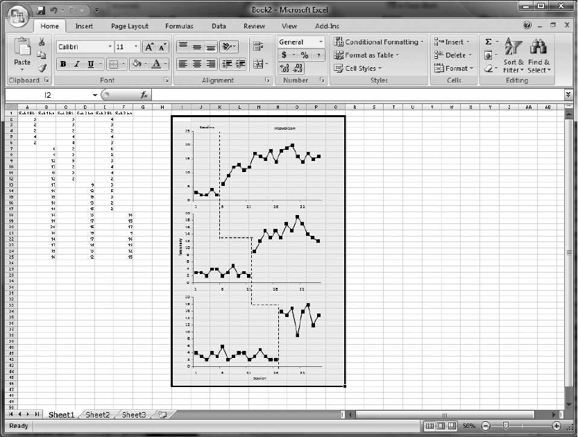
Figure 6. Sample data and early graphs of a multiple baseline design.

286 MARK R. DIXON et al.

the INSERT tab and select LINE

GRAPH, and then the fourth option in

the line graph submenu, titled LINE

WITH MARKERS. Carr and Burk-

holder (1998) described a process by

which you can copy your first graph

and paste the identical graph immediate-

ly below it, after which you change the

data series of the second graph to the

data representing the 2nd participant.

We have already described the utility and

process of saving a graph as a template

for later use with new data. However, the

existing graph we have created is in need

of modifications before it is ready to be

converted into a template.

3. Begin the modifications by deleting the

legend by left-clicking on it once and

pressing the DELETE key. Delete the

grid lines by clicking once on one of the

grid lines, which will highlight all of

them, and then press the DELETE key.

4. At this time we can also remove the

border and fill colors from the chart area

and plot areas, as described for previous

graphs. Depending on your preference

settings in Excel 2007, the graph may or

may not have a background by default.

5. You may wish to edit the line colors and

marker styles at this time. To do so,

right-click on the data series you wish to

edit. From the FORMAT DATA SE-

RIES window, select MARKER OP-

TIONS and the suboption BUILT-IN.

Choose a marker type you wish to use.

With the BUILT-IN option selected, you

may choose the type and size of marker

you wish to use on the graph.

6. Change the line color by selecting the

option LINE COLOR, selecting the

option SOLID LINE, and, using the

drop-down menu for color, choose the

color you wish to use. You may also need

to change the marker fill color and

marker line color as well. Once all three

options are set to the same color, press

CLOSE to return to the graph. To make

the same changes to your other data

series, repeat the steps previously de-

scribed.

7. As you may notice, the x -axis tick-mark

labels range from 1 to 24 in our example,

which appear to be quite cumbersome. In

Excel 2007, we can easily alter this x-axis

display by selecting the LAYOUT tab

under the chart tools, and under the

LAYOUT tab in the fourth panel, select

the AXIS option. Then select the PRI-

MARY HORIZONTAL AXIS and then

select the last option, MORE PRIMA-

RY HORIZONTAL AXIS OPTIONS.

8. From the FORMAT AXIS window,

select the AXIS OPTIONS, and then

change the intervals between tick marks

from 1 to 5. Then, select SPECIFY

INTERVAL UNIT and change this

from 1 to 5. Now click the CLOSE

button to return to the graph.

9. There are various other options you may

wish to explore to edit other character-

istics of the axes. For now, the ones

described above will suffice. Some of the

new features of Excel 2007 include

changing the axis types to dates, present-

ing the axis in 3-D formats, and aligning

the text in various directions and angles.

10. Before we save this edited chart as a

template, we must decide whether we

wish to add phase-change lines here on

the individual graphs. Unlike the other

types of graphs described in this task

analysis, the MBD graph will require

phase-change lines that cross multiple

graphs; however, this is not possible

when one draws the lines directly on a

graph, as described previously for the

reversal design graphs, because lines will

not extend beyond the border of the

chart area. We suggest that for MBD

graphs you forgo drawing phase-change

CREATING DESIGN GRAPHS 287

lines directly on graphs and wait until all

graphs are completed and aligned to add

phase-change lines. We will describe this

process below.

Saving the Graph as a Template and Using the

Saved Template for Subsequent Graphs

1. The graph is now ready to be saved as a

template. Save the graph as a template as

previously described, using the text ‘‘Mul-

tiple Baseline’’ for the file name when

saving the template file.

2. To create the graph for the 2nd partici-

pant, highlight that participant’s data,

select INSERT, OTHER CHARTS from

the CHARTS panel, and select the last

option ALL CHART TYPES.

3. From the INSERT CHART window,

select the first option TEMPLATES and

the newly created ‘‘Multiple Baseline’’

option displayed under MY TEM-

PLATES. Select OK and return to the

graph. You will now see a second graph

with identical formatting, but with the

data series for the 2nd participant. Repeat

this process for the 3rd participant’s data.

Aligning and Grouping the MBD Graphs

1. At this point, you will have three graphs

of different data that are identically

formatted. To arrange them into a

multiple baseline display, align the

graphs horizontally and vertically so that

each subsequent participant’s graph is

below the previous participants’ graphs.

Once all three graphs are aligned verti-

cally and horizontally, we can group all

three graphs so that if we need to move

the graphs on the spreadsheet in the

future, we will simply have to move one

item instead of three.

2. To group all three graphs, hold down the

Ctrl key and left-click once on the chart

area of each graph. This should select all

three graphs. Now right-click and select

the GROUP option. Now you should be

able to select and reposition all three

graphs as one item by clicking on the

area surrounding the three graphs. If

completed properly, you should see a box

around all three graphs like the one

displayed in Figure 6.

3. At this point we need phase-change lines

added to the graphs, and as stated

previously, these lines need to cross

multiple graphs. To accomplish this,

make sure that you have selected some-

where on the spreadsheet outside the

graphs by clicking on any cell away from

the graphs. To draw the first line, click

on the INSERT tab of the main menu,

and in the ILLUSTRATIONS panel

select the SHAPES option and select

the first LINE option displayed.

4. With the mouse draw a vertical line in an

area of the spreadsheet away from the

graphs. You can ensure the line will be

perfectly vertical (or horizontal) if you

hold down the shift key while drawing

the line. Change the color, solid or

dashed style, and other options of the

line as described previously, then with

the mouse reposition the line over the

graphs to separate phases of the graph.

You may need to extend the length of the

line by either clicking and dragging on

the ends of the line or, once the line has

been selected, you may click on the

FORMAT option on the menu, then

locate the SIZE panel. The length of the

line can be adjusted in specified incre-

ments by adjusting the SHAPE WIDTH

option (i.e., the second numeric up-down

box in the SIZE panel).

5. You can repeat these steps for the

remaining phase-change lines, or you

may simply copy, paste, and adjust the

just-completed line, as described previ-

ously.

288 MARK R. DIXON et al.

6. In most MBD graphs, single x- and y-

axis labels are used to describe all

participants’ data. To create single x -

and y-axis labels, you will need to move

outside the graphs and create the labels

on the spreadsheet, using text boxes.

7. To do this, click on a spreadsheet cell

outside the charts, click on the INSERT

tab, and in the panel TEXT, select the

first option (TEXT BOX), and then draw

your text box on the spreadsheet away

from your graphs.

8. Type in the desired x -axis label. Follow-

ing our example, enter the text ‘‘Ses-

sion.’’

9. To move the x-axis label below the 3rd

participant’s graph, select it by left-

clicking on it once. While holding down

the left mouse button, drag it to the

bottom of the 3rd participant’s graph.

10. Repeat this process for the y-axis label.

Enter the text ‘‘Frequency’’ for the y-axis

label.

11. You may need to rotate the y-axis label

270 degrees. With the text box highlight-

ed, right-click and select FORMAT

SHAPE from the options that appear.

From the FORMAT SHAPE window,

select the last option, TEXT BOX, the

suboption TEXT DIRECTION, and the

drop-down menu option ROTATE 270

DEGREES. Select CLOSE to return to

the spreadsheet.

12. Resize the text box and position it to the

left of the 2nd participant’s y-axis values.

13. Remove the border and background

color of the text boxes, as described

previously.

14. Repeat the process described previously

for reversal design graphs to create labels

for the different phases. Position the

resulting text boxes above the data series

of the 1st participant. The resulting

MBD graph should look similar to the

one depicted in Figure 7.

Exporting the Graph into Another Program

Even though instructing readers in the use of

Excel 2007 to create graphs is the ultimate goal

of this paper, displaying those graphs only in

Excel 2007 is rarely the ultimate goal of those

who create graphs. Ultimately, we will present

graphs of our data elsewhere, such as word

processing (e.g., Microsoft Word

) or presen-

tation (Microsoft PowerPoint

) software. The

point is that ultimately we will need to know

how to transport a finished graph from Excel

2007 to other applications.

1. To export your final product from Excel

2007 into other applications, use your

mousetohighlighttheentirefigure

consisting of all three graphs by left-

clicking on a cell to the left and above all

aspects of the graphs. Then while holding

down the left mouse button, drag to a cell

to the right and below all aspects of the

graphs. Make sure to include the x- and y-

axis labels. When highlighted, the area

should look like Figure 7. With all of the

elements highlighted, right-click and

choose the COPY option. When the

graph to be transferred is selected, the

simplest option is to open the desired

program, right-click in the area of your

new document you wish to display the

graph in, and select PASTE. A safer

option that can be used when transferring

graphs to Word or PowerPoint is to use

the Paste as Picture option located under

the PASTE SPECIAL options of either

Word or PowerPoint. This option gener-

ally does a better job of retaining all

features of a graph; however, the user will

lose the ability to modify any features of

the graph in its new location except for its

size.

2. Excel 2007 has additional features for

transporting your graphs to other pro-

grams. With the figure highlighted, select

the Office 2007 icon in the top left corner

of the screen. This icon is titled the

CREATING DESIGN GRAPHS 289

OFFICE BUTTON, and will display

options such as PREPARE, SEND, and

PUBLISH. These three options will allow

you to do many things, such as e-mail the

whole spreadsheet or figure, publish it as

an independent document, and prepare it

for final encryption. If the reader owns a

copy of Adobe Acrobat, a SAVE AS

option will allow automatic conversion of

the figure into a .pdf file. Even if the

reader does not own Acrobat, there are

free add-ins available for download from

Microsoft’s Web site (http://www.microsoft.

com/downloads/), including the Flash-

Paper Toolbar and the Microsoft Save as

PDF or XPS that make saving spread-

sheets and figures as .pdf and .xps files a

simple option.

Improvements in the Visual Formatting

of Spreadsheets

Thus far we have described the basic

components of Excel 2007 that you should be

familiar with to create common single-subject

design graphs. To illustrate these features we

have employed relatively simple data sets.

However, real data often result in relatively

busy spreadsheets. To prevent graphs from

cluttering your spreadsheet, you may transfer

them to a separate spreadsheet within the same

Excel 2007 file. To do this, simply highlight the

graph, right-click, and select COPY. Locate the

tabbed spreadsheet labels in the bottom left

corner of the work space and select SHEET 2

(or any other sheet). When SHEET 2 has been

highlighted, right-click and select PASTE. The

graph will now appear on the new spreadsheet.

Figure 7. The completed multiple baseline design graphs with the all of the graphs highlighted.

290 MARK R. DIXON et al.

Using a new separate spreadsheet is even more

helpful with multiple graphs that may need very

careful alignment.

Excel 2007 offers many either new or

improved features that make the visual display

of spreadsheets more easily customizable. Ear-

lier, when we described how to set up a

spreadsheet, we mentioned that users may wish

to color code cells manually to correspond to a

given phase (e.g., baseline, treatment). Excel

2007 features an interface for applying condi-

tional formatting rules to cells in a spreadsheet

that is much improved over previous versions of

the software. Given the color-coding example

we just mentioned, one could apply a rule that

would automatically change either the text color

or the highlight color of a cell or group of cells

based on the text entered. One could also apply

rules based on some function of a series of

values in a group of cells. One can apply

conditional formatting rules that change text or

highlight colors of the top 10 scores in a series

of values, the top 10% of scores in a series of

values, the bottom 10% of scores in a series of

values, only those values above a mean of a

certain series of values, or only those values

below a mean of a certain series of values.

Multiple rules can be set for a block of cells so

that more than one of these types of rules can be

applied, with the order of which rules to apply

first left modifiable. It is not hard to see that the

possibilities can easily get complicated.

To illustrate some of the ways that these

features could be applied, we will use the

example of a spreadsheet set up to display data

in a type of research design most readers should

be familiar with, the changing-criterion design.

Consider a scenario in which one wants to

increase the number of mands emitted by a

client per session. One may wish to take

baseline data for a number of sessions and then

apply an initial criterion for advancement

through a training protocol. A simple way to

set up a spreadsheet might be to place a header

in the first column (Column A) for the phase

and a header in the second column (Column B)

for the frequency of mands. Data entered in the

first column would consist of text correspond-

ing to phase (BL for baseline, TXCT1 for the

first training criterion, TXCT2, for the second,

etc., for all remaining criterion levels), and data

in the second column would consist of the

frequency of mands emitted per session or

observation. To serve as a more salient visual

reference, you might wish to highlight the cells

in the phase column with a specific color based

on the phase entered. The following instruc-

tions illustrate this process.

1. Click on Column A to highlight the

entire column.

2. From the main menu at the top of the

screen make sure the HOME tab is

selected and locate the CONDITIONAL

FORMATTING option from the

STYLES panel at the top of the screen.

3. Click on CONDITIONAL FORMAT-

TING and from the resulting option

select the NEW RULE option.

4. In the resulting NEW FORMATTING

RULE dialogue box, select the FORMAT

ONLY CELLS THAT CONTAIN option

from the SPECIFIC RULE TYPE box.

5. In the EDIT THE RULE DESCRIP-

TION box, select the SPECIFIC TEXT

option from the first drop-down box,

select the CONTAINING option from

the second drop-down box, and in the

text box on the right enter the text you

want to enter in the cells for the first

phase of the study (BL for baseline).

6. Click on the FORMAT button to open

the FORMAT CELLS dialogue. From

this dialogue, click on the FILL tab and

select the color you wish the cells to be

highlighted with, then click the OK

button to return to the NEW FORMAT-

TING RULE dialogue box. Click on the

OK button to finalize the new rule.

7. Repeat the steps above to add additional

rules for highlighting the cells in the

CREATING DESIGN GRAPHS 291

phase column with different colors when

text for the other phases is entered (i.e.,

TXCT1, TXCT2).

8. Test the results of the rules by entering

the text ‘‘BL’’ in the first five cells in the

phase column, the text ‘‘TXCT1’’ in the

next 5 to 10 cells, and the text ‘‘TXCT2’’

in the next 5 to 10 cells.

Now assume you collect baseline data for five

sessions and obtain frequencies of 10, 15, 11,

12, and 14 mands per session for your baseline

observations, for a mean of 12.4 mands per

session. At this point, we might begin to

implement a training protocol, and we might

set a criterion of observing at least four of five

consecutive sessions with frequencies equal to or

greater than 25% over the mean baseline rate

before moving to the next criterion level. As we

enter data for these sessions in the TXCT1

phase, we want any values that meet the

criterion to be displayed in red text so we could

quickly visually determine if four of the last five

sessions have met the current criterion level.

Again, we can add rules with the conditional

formatting options to accomplish this.

1. In Cell E1, enter the text ‘‘Criterion Level 1.’’

2. In Cell F1, enter the following text to

create a formula to calculate the criterion

level: ‘‘51.25 * AVERAGE(B2:B6).’’

This formula calculates the mean of the

five baseline observations and multiplies

it by 125% to obtain the first criterion

level.

3. We also want to add in the second

criterion level. In Cell E2, enter the text

‘‘Criterion Level 2.’’

4. We want the second criterion level to be

25% greater than the previous level, so in

Cell F2 enter the following formula

‘‘51.25 * F1.’’

5. Select all the cells in the frequency

column by clicking on Column B.

6. Click on the CONDITIONAL FOR-

MATTING tab in the STYLES panel

and select the NEW RULE option.

7. In the resulting NEW FORMATTING

RULE dialogue box, select the FOR-

MAT ONLY CELLS THAT CON-

TAIN option in the SELECT A RULE

TYPE box.

8. In the EDIT THE RULE DESCRIP-

TION box, make sure that CELL VAL-

UE is selected in the first drop-down box

and that GREATER THAN OR

EQUAL TO is selected in the second

drop-down box.

9. In the third box you can either enter a

specific value or select a value from a

specific cell in the spreadsheet by clicking

on the selection icon on the right side of

the box, selecting the appropriate cell in

the spreadsheet (in this case, Cell F1, in

which we entered the formula for calcu-

lating Criterion Level 1) containing the

value you want to use, and clicking on the

selection icon again to return to the EDIT

FORMATTING RULE dialogue box.

10. Click on the FORMAT button to open

the FORMAT CELLS dialogue box,

select the FONT tab, select red from the

COLOR drop-down box in the middle of

thedialoguebox,andclickontheOK

button to return to the EDIT FORMAT-

TING RULE dialogue box. Click the OK

button to complete the rule.

11. Repeat Steps 6 to 10 to create another

rule to make all values greater than or

equal to the second criterion level a

different color of text, except in Step 7

select Cell F2 and in Step 10 select a

color other than red.

12. Finally, to test if the new rules work,

enter numerical values into Cells B7 and

B27. Values between the two criterion

levels should be displayed in red, and

those greater than or equal to the second

criterion level should be displayed in the

color you chose in Step 11.

The steps described above only begin to

scratch the surface of the formatting options

292 MARK R. DIXON et al.

available in Excel 2007. In addition to the text

and highlighting options described in the

preceding section, the conditional formatting

option has many more features and additional

rules that can be applied to spreadsheets. Users

who wish to explore additional options on

their own may benefit by consulting the help

screen in Excel 2007. By clicking on the

question mark within the blue circle in the

upper right corner of Excel 2007 and typing

‘‘conditional formatting’’ into the resulting

search box, one can find links to demonstra-

tions and downloads from Microsoft that may

help to illustrate the use of many of these

additional options.

SUMMARY

Microsoft’s Excel 2007 spreadsheet program

remains useful for behavior analysts desiring to

create single-subject design graphs. We have

described the necessary steps for a few common

graph types using Excel’s latest version, and

with slight modifications, many others are

possible. In the present article we have only

scratched the surface of the graphing and data

analysis possibilities in Excel 2007. Future

explorations might include tutorials for calcu-

lating interobserver agreement, developing

macros for data analysis, or the construction

of other types of graphical displays.

REFERENCES

Carr, J. E., & Burkholder, E. O. (1998). Creating single-

subject design graphs with Microsoft Excel

. Journal

of Applied Behavior Analysis, 31, 245–251.

Cooper, J. O., Heron, T. E., & Heward, W. L. (2007).

Applied behavior analysis (2nd ed.). Upper Saddle

River, NJ: Merrill/Prentice Hall.

Received May 2, 2007

Final acceptance November 12, 2008

Action Editor, James Carr

CREATING DESIGN GRAPHS 293